Mathematical Backgrounds
Notation
- $\mathbb{R}$ - field of real, $\mathbb{R}_{+}=\{\alpha\in \mathbb{R}: \alpha>0\}$;
- $|x|=\sqrt{x^{\top}x}$ is the Euclidean norm in $\mathbb{R}^n$, $x\in \mathbb{R}^n$
- $P\succ 0$ means $P=P^{\top}\in \mathbb{R}^{n\times n}$ is a positive definite symmetric matrix ($\prec 0, \succeq 0, \preceq 0$)
- $\mathbf{d}(s)=e^{ sG_\mathbf{d}}, s\in \mathbb{R} $ is a linear dilation in $ \mathbb{R}^n $ with an anti-Hurwitz matrix $ G_\mathbf{d}; $
- $\|x\|\!=\!\sqrt{x^{\top} Px}$ is the weighted Euclidean norm such that $P\!\succ\! 0, PG_\mathbf{d}\!+\!G_\mathbf{d} ^{\top} P\succ 0$;
- $S=\{x\in \mathbb{R}^n: \|x\|=1\}$ is the unit sphere;
- $\|\cdot\| _\mathbf{d}$ is the canonical homogeneous induced by $\|\cdot\|$(see below);
- $\mathcal{H}_\mathbf{d} ( \mathbb{R}^n)$ - a set of all $ \mathbf{d}$ -homogeneous functions $ \mathbb{R}^n \mapsto \mathbb{R}$ (see below);
- $\mathcal{F}_\mathbf{d} ( \mathbb{R}^n)$ be a set of all $ \mathbf{d}$ -homogeneous vector fields $ \mathbb{R}^n \mapsto \mathbb{R}^{n}$;
- $\deg_\mathbf{d}$ (f) - homogeneity degree of $f$.
1. Problems Under Consideration
The classical problems of the control systems theory
- state/output stabilization of a system
- state estimation of a system
are considered under additional constraint of a finite or a fixed-time response (see below) of the system. Solutions to these problems are going to be developed based on the generalized homogeneity surveyed in this chapter. Let us first theoretical formulations of the mentioned control/estimation problems.
1. 1 Stabilization Problem
$\textbf{Model of control system:}$$$ \quad \quad \dot x(t)=Ax(t)+Bu(t), \quad t>0\quad \quad \quad (1) $$
- $x(t)\in \mathbb{ R } ^n$ is the system state
- $u(t)\in \mathbb{ R } ^m$ is the control input (can be modified as need)
- $A\in \mathbb{ R } ^{n\times n}$ and $B\in \mathbb{ R } ^{n\times m}$ are $\underline{known}$ matrices
Asymptotic Stabilization by a Feedback Law
The problem is to design $u : \mathbb{ R } ^n \mapsto \mathbb{ R } ^m$ such that the system$$ \dot x(t)=Ax(t)+B u (x(t)) $$
is asymptotically stable $\Rightarrow $ $$x(t)\to 0 \quad \text{ as } \quad t\to+\infty$$
$$ $$
Finite-time Stabilization by a Feedback Law
The problem is to design $ u: \mathbb{ R }^n \mapsto \mathbb{ R }^m$ such that the system
$$ \dot x(t)=Ax(t)+B u(x(t)) $$ is finite-time stable $\Rightarrow$ $$ \forall x(0)\in \mathbb{ R }^{n}, \quad \exists T=T(x(0))\geq 0 \quad : \quad x(t)=\mathbf{ 0}, \quad \forall t\geq T $$
$$ $$
Fixed-time Stabilization by a Feedback Law
The problem is to design $ u: \mathbb{ R }^n \mapsto \mathbb{ R }^m$ such that the system $$ \dot x(t)=Ax(t)+B u(x(t)) $$ is fixed-time stable $\Rightarrow$ $$ \exists T_{\max}>0 \quad : \quad x(t)=\mathbf{ 0 }, \quad \forall t\geq T_{\max}, \quad \forall x(0)\in \mathbb{ R }^{n} $$
A stabilization of an output $y=Cx$ is a particular case of the above problems.
1. 2 State Estimation Problem
$\textbf{Model of the system:}$
$$\quad \quad \quad \dot x(t)=Ax(t)+p(t), \quad y(t)=Cx(t) \quad \quad \quad (2)$$
- $x(t)\in \mathbb{ R } ^n$ is the system state (${\color{red}{unknown}}$)
- $p(t)\in \mathbb{ R } ^n$ is the exogenous input ($\underline{can \; be \; measured \; online}$)
- $y(t)\in \mathbb{ R } ^k$ is the measured output
- $A\in \mathbb{ R } ^{n\times n}$, $B\in \mathbb{ R } ^{n\times m}$ and $C\in \mathbb{ R } ^{k\times n}$ are $\underline{known}$ matrices
Asymptotic Observer
The problem is to design a system (asymptotic ${\color{red}{observer}}$ )
$$ \dot z(t)=f(z(t),p(t),y(t)), \quad \quad f:\mathbb{ R } ^n\times \mathbb{ R } ^n \times \mathbb{ R } ^k \mapsto \mathbb{R}^n $$ such that $ \|z(t)-x(t)\| \to 0 \quad \text{ as } t\to +\infty $
$$ $$
Finite-time Observer
The problem is to design a system (finite-time observer)
$$ \dot z(t)=f(z(t),p(t),y(t)), \quad \quad f:\mathbb{ R } ^n\times \mathbb{ R } ^n \times \mathbb{ R } ^k \mapsto \mathbb{ R } ^n $$
such that $ \forall x(0)\in \mathbb{ R } ^{n},\quad \exists T=T(x(0))\geq 0 \quad : \quad \|z(t)-x(t)\| = 0, \forall t\geq T $
$$ $$
Fixed-time Observer
The problem is to design a system (fixed-time observer)
$$ \dot z(t)=f(z(t),p(t),y(t)), \quad \quad f:\mathbb{ R } ^n\times \mathbb{ R } ^n \times \mathbb{ R } ^k \mapsto \mathbb{ R } ^n $$
such that $\quad \exists T_{\max}>0 \quad : \quad \|z(t)-x(t)\| = 0, \quad \forall t\geq T_{\max}, \quad \forall x(0)\in \mathbb{ R } ^{n}.$
2. From Linearity to Homogeneity in Control Systems Design
The basic idea of the homogeneity based control/observer design is an expansion of linear methods/algorithms of (asymptotic controllers/observers) design to nonlinear systems such that finite/fixed-time stability can be provided by means of the tuning of the so-called homogeneity degree. This section explains the basis intuitions behind the mentioned idea.
2. 1 Homogeneity is a Dilation Symmetry
In mathematics, an invariance of some characteristics of an object with respect to a certain group of transformations is known as a symmetry. The simplest example of a symmetry is the invariance of geometric figures with respect to a rotation or a dilation
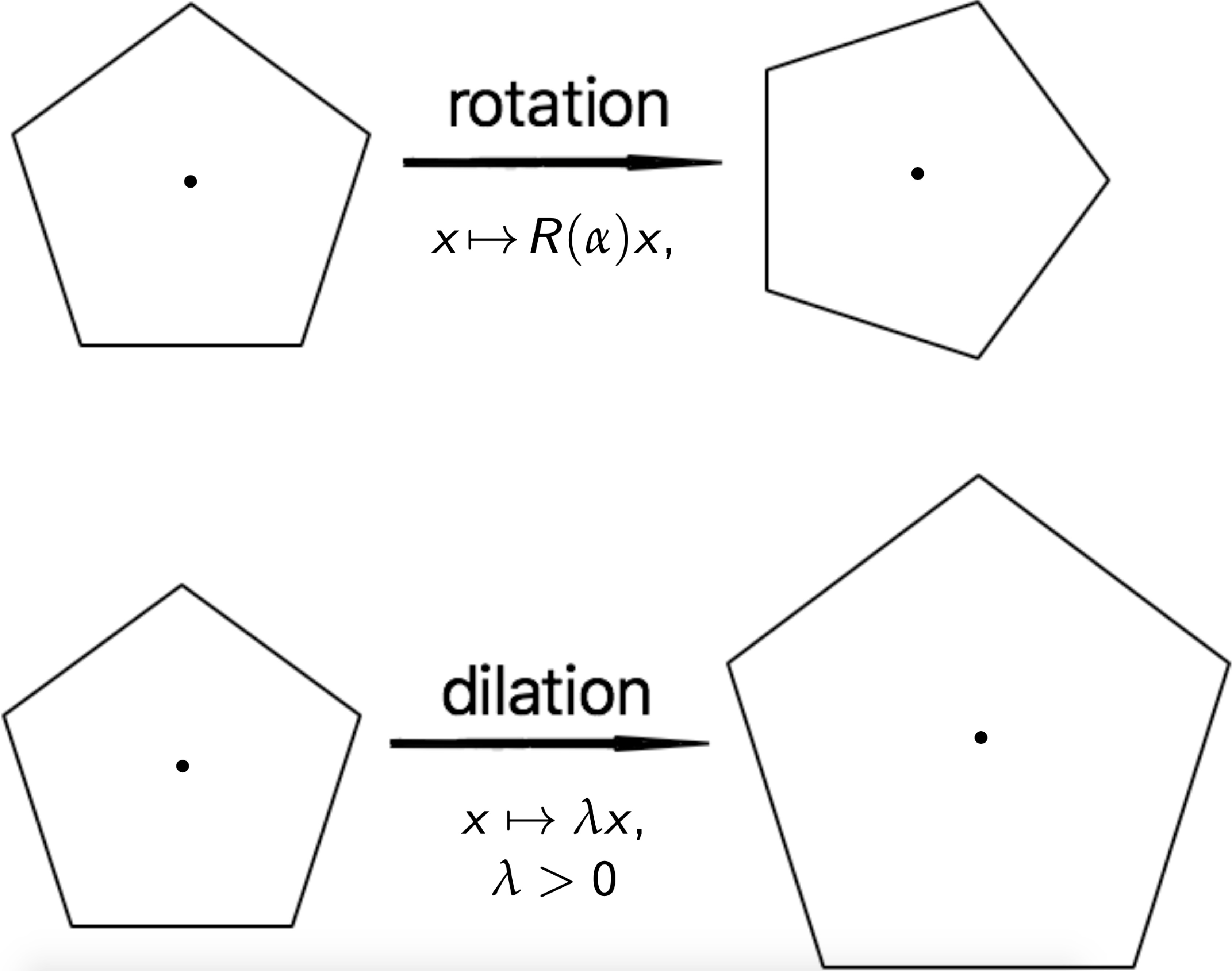
Rotation and dilation symmetries of the figure
$$ $$
$f$ is linear $\Leftrightarrow $ ${\color{BlueViolet}{f(\lambda x)=\lambda f(x)}}$ & ${\color{blue}{f(x+y)=f(x)+f(y)}} $ & ${\color{Maroon}{f(-x)=-f(x)}} $$$ $$
$\textit{Example}$: $f(x)=x_1+x_2$, where $x\!=\!(x_1,x_2)^{\top}$
$$ $$
Standard Homogeneity $ (Leonhard \;\; Euler, \;\; 18th \;\; century) $
$$ $$
$x\mapsto \lambda x \; ({\color{BlueViolet}{standard\; dilation}}) $ $f(\lambda x)=\lambda^{\nu} f(x), \;\; \;\; \forall s,x \;\; \;\; ({\color{BlueViolet}{symmetry}})$
$\lambda>0 $ - scaling factor $\nu\in \mathbb{ R }$- homogeneity degree
$$ $$
$\textit{Example}$: $f(x)=x_1x_2+x_2^2$ is standard homogeneous of degree 2:$f(\lambda x)=\lambda^{2}f(x)$
$$ $$
Generalized Homogeneity $ ( $ Zubov, 1958 [ 24 ] ; Kawski, 1991 [ 6 ] $ ) $
$$ $$
$x \to\mathbf{d}(s)x $ $ ({\color{BlueViolet}{generalized \;\; \;\; dilation}})$ $ f(\mathbf{ d }(s)x)=e^{\nu s} f(x),$ $ ({\color{BlueViolet}{symmetry}})$$ {\color{BlueViolet}{Limit \;\; property}}: \;\;\; \lim\limits_{s\to -\infty}\|\mathbf{ d }(s)x\|\!=\!0, \;\; \;\; $ $ \lim\limits_{s\to +\infty}\|\mathbf{ d } (s)x\|\!=\!+\infty,\;\; \forall x\!\neq\! \mathbf{ 0 } $
$\textit{Example}$: $\mathbf{d}(s)=\left(\begin{smallmatrix}e^{2s} & 0\\ 0 & e^s\end{smallmatrix}\right)$, $f(x)=x_1+x_2^2$ is $\mathbf{d}$-homogeneous:$\mathbf{d}(s)x=\left( e^{2s}x_1,\; e^{s}x_2\right)^{\top} \quad \text{ and } \quad f(\mathbf{d}(s)x)=e^{2s}f(x)$
$$ $$
$$ $$
The HPC toolbox deals only with ${\color{red}{linear \;\; dilations}} $ in $\mathbb{ R }^n$.
$$ $$
Linear Dilation $ ($see e.g. Polyakov , 2019, [ 14 ] - [ 15 ] )
$$ $$
A continuous linear $\textbf{dilation}$ in $\mathbb{ R } ^n$ is a matrix-valued function given by
$ \mathbf{ d } (s)=e^{sG_{\mathbf{ d } }}=\sum\limits_{i=0}^{+\infty}\tfrac{s^iG_{\mathbf{ d } }^i}{i!}, s\in \mathbb{ R } $
where $G_{\mathbf{ d } }\in \mathbb{ R } ^{n\times n}$ is an $\textit{anti-Hurwitz matrix}$ called a $\textbf{generator}$ of $\mathbb{ R } $.
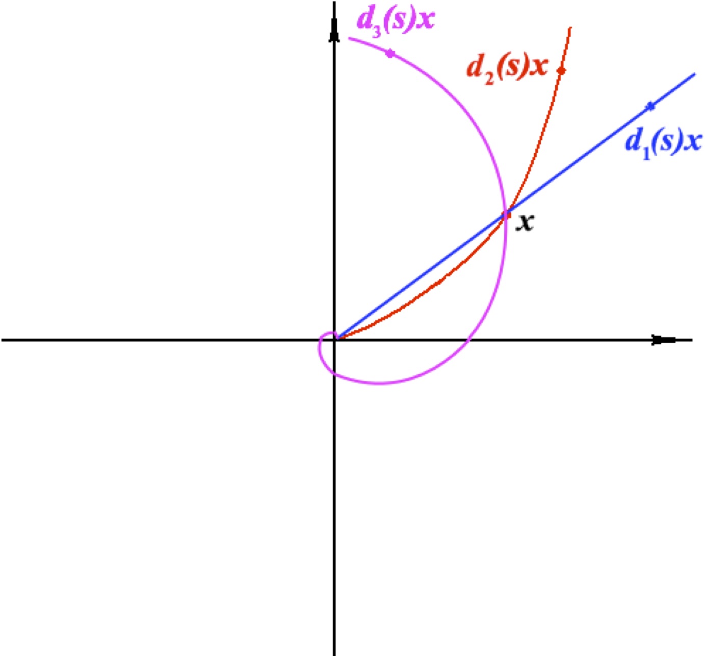
| $\textbf{Standard dilation}:$ $ {\color{blue}{\mathbf{ d } _1(s)=e^{s}I,}}\;\;\; G_{\mathbf{ d } }=I\in \mathbb{ R } ^{n\times n}$
|
 |
|
| $\textbf{Weighted dilation}:$ $ {\color{red}{\mathbf{ d } _2(s)= \texttt{diag}\{e^{r_i s}\} }}\;\;\; G_{\mathbf{ d } }= \texttt{diag}\{r_i\}\succ 0 $
|
||
| $\textbf{Linear dilation}:$ ${\color{magenta}{\mathbf{ d }_3(s)=e^{sG_d},}} \;\;\;G_{\mathbf{ d } }\;\;\; is \;\;\;anti-Hurwitz $
|
2. 2 Properties of Homogeneous Systems
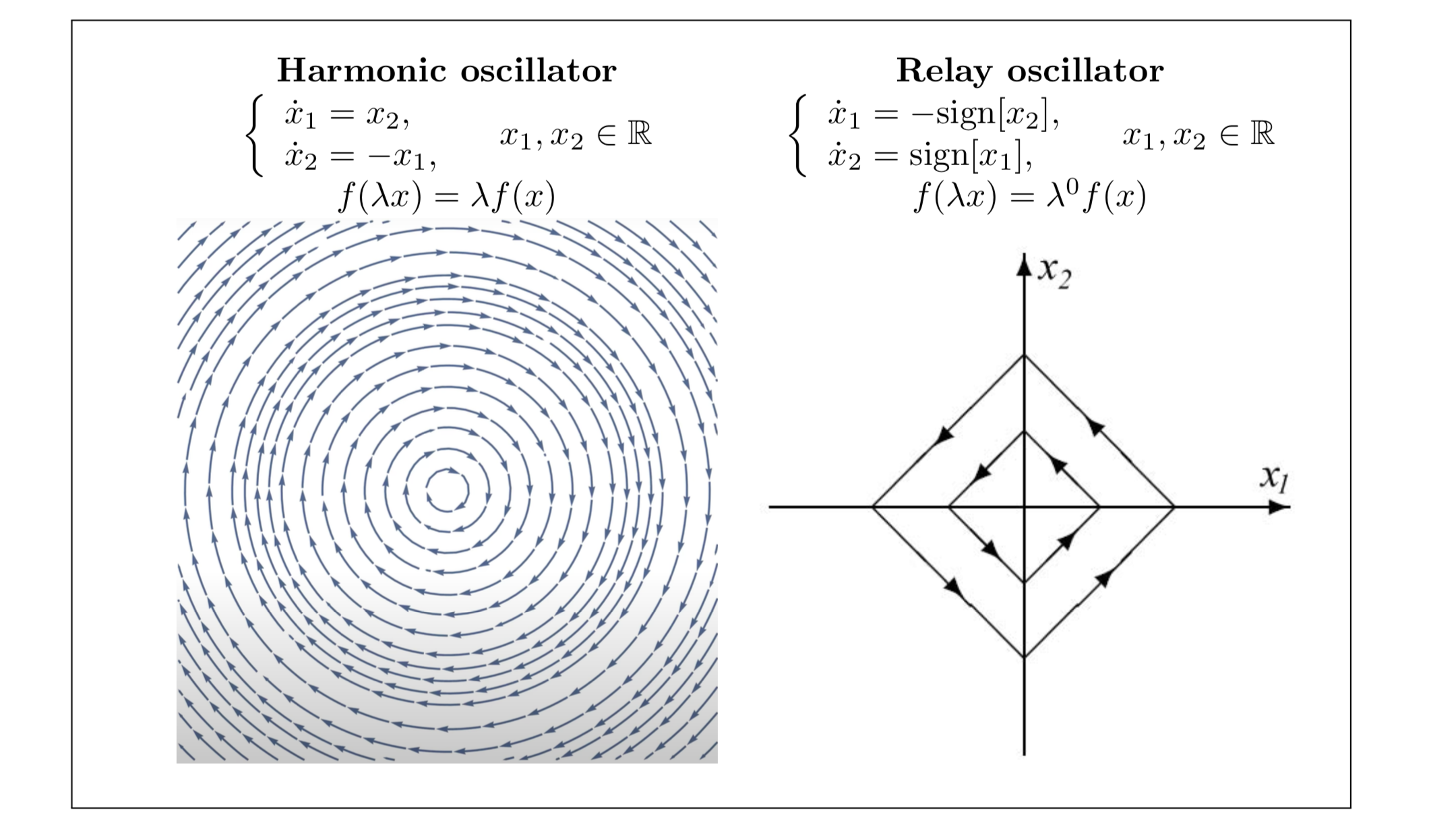
Homogeneity (dilation symmetry) of a function is inherited by any other mathematical object induced by this function: the derivatives of the homogenous functions are homogeneous as well, solutions of differential equations with homogeneous right-hand side are symmetric, etc. Indeed, for example, see below the dilation symmetry of solutions of two standard homogeneous systems (harmonic and relays oscillators) with respect to scaling of initial conditions.
| $\textbf{Linear System} \;\; \\ \dot x=Ax,\;\; x(0)=x_0\;\; \\ A\in \mathbb{ R } ^{n\times n} is \;\; a \;\; matrix$
|
$\textbf{Homogeneous
System} \;\; \\ \dot x=f(x),\;\; x(0)=x_0 \;\;\\ {\color{blue}{f(\mathbf{d} (s)x)=e^{\mu s}\mathbf{d} (s)f(x)}} $ |
|
|---|---|---|
$\textbf{Trajectory Scaling} $ |
$x(t,e^s x_0)\!=\!e^s x(t,x_0)$ |
$\!x\!\left(t,\mathbf{d} (s)x_0\right)\!=\!\mathbf{d} (s)x(e^{\mu s}t,x_0)\!$ |
$\textbf{Local} \Leftrightarrow \textbf{Global} $ |
$\checkmark$ |
$\checkmark$ |
$\textbf{Invariance}$ $\Leftrightarrow \textbf{Stability} $ |
$\checkmark$ |
$\checkmark$ |
$\textbf{Stability} \Rightarrow
\textbf{Robustness} \\ (Input-to-State\;\; Stability) $ |
$\dot x=Ax+Dw \\ w\in L^{\infty} $ |
$\dot x=f(x,w) \\ w \in L^{\infty}$ |
$\textbf{Convergence Rate} $
|
$ Exponential $ |
$+ \;\; Finite/Fixed-time \; {\color{blue}{(\mu\neq 0)} }$ |
$\textbf{Lyapunov Function} $
|
$A \; weighted \; Euclidean \; norm \\ V=\sqrt{x^{\top} P x}, \quad P\succ 0$ |
$A\;\; homogeneous \;\; norm \;\; \\ V(\mathbf{d} (s)x)=e^{s} V(x)$ |
$\textbf{Consistent discretization} \\ (preserves\;\; convergence \;\;rate) $ |
$\checkmark $ $Exponential $ |
$\checkmark $ $+\;\; Finite/Fixed-time \;\; {\color{blue}{(\mu\neq 0)}}\\ $ |
$$ $$
Question
$ \textit{Is there any potential advantage of a homogeneous system versus a linear one?}$
2. 3 Linearity vs Homogeneity
-
$\textbf{Convergence rates of homogeneous and locally homogeneous systems:} $
$\left\{ \begin{array}{l} \dot x(t)=u(t), \\ x(0)=x_0, \end{array} \right. \quad x,u\in\mathbb{ R }.$- $\textbf{Exponential stability} \;\; $ ( $\textit{ Lyapunov 1892 }$, [8] ):
-
- $ u(t)=-x(t) $
-
- $ {\color{blue} { x(t)=e^{-t}x_0 \to 0 \text{ if }t\to+\infty} } $
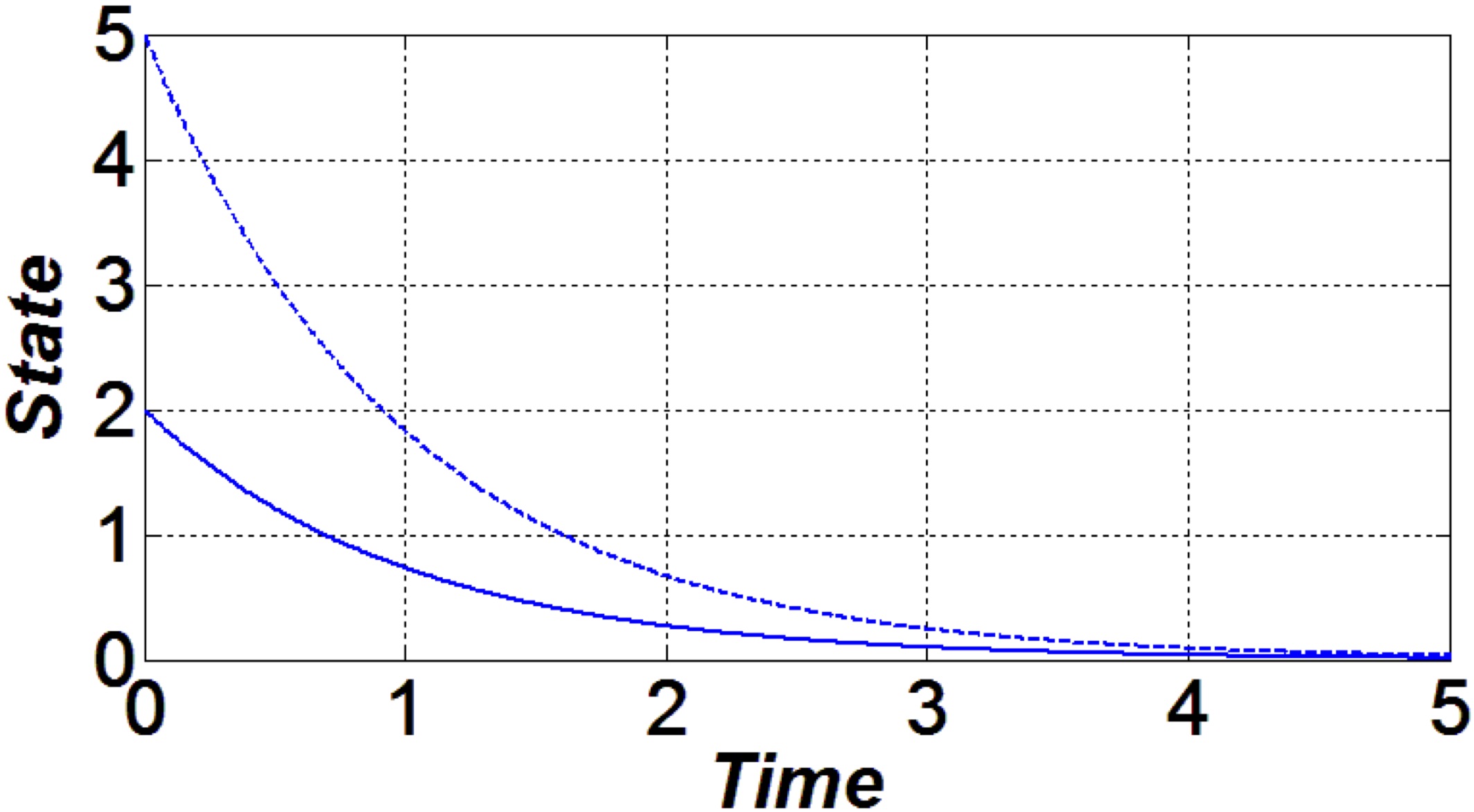
- $\textbf{Finite-time stability} \;\; ( $ $ \textit{Roxin 1966}, [21] $ ):
-
- $ u(t)=- \texttt{sing}(x(t)) $
-
- $ {\color{blue} {x(t)= 0} } \text{ for } {\color{blue} {t\geq \|x_0\|}} $
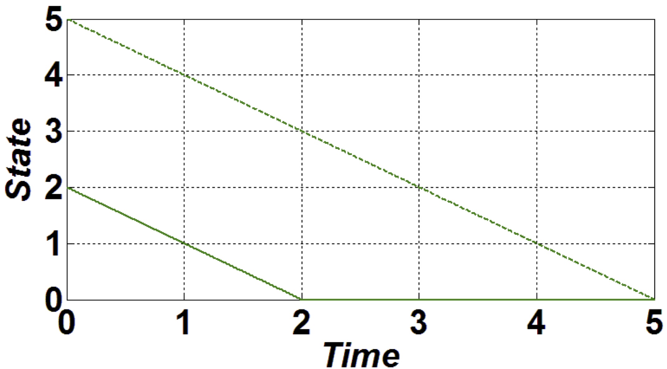
- $\textbf{Fixed-time stability} \;\; ( $ $ \textit{Polyakov 2012}, [13] $ ):
-
- $ u(t)\!=\!-\left(|x(t)|^{\frac{1}{2}}\!+\!|x(t)|^{\frac{3}{2}}\right)\! \texttt{sing}(x(t))$
-
- $ {\color{blue} {x(t)=0}} \text{ for } {\color{blue} {t\geq \pi}} \;\;\;\; {\color{red}{independently \;\; of \;\;\;\; x_0}} $
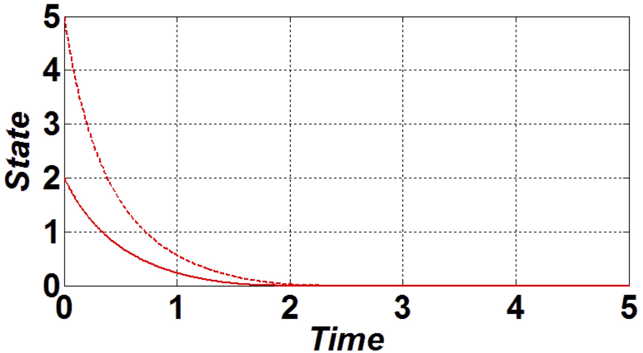
Conclusion I
Homogeneous system may have faster convergence than linear one. - $\textbf{Robustness issues of homogeneous systems:} $
Model of system $\dot x=\lambda x+u, \\ {\color{red} {where \;\; \lambda>0 \;\; is\; unknown \; constant}}$ $\dot x=u+g(t), \\ {\color{red} {where \;\;\;\; g(t) \;\;\;\; is \;\;\;\; unknown \;\;\;\; but }}\\ {\color{red}{bounded \;\;\;\; function \;\;\;\; |g(t)|\leq \bar g.}} $ Control aim $stabilize \;\;\;\; x\;\;\;\; to \;\;\;\; 0$ $stabilize \;\;\;\; x\;\;\;\; to \;\;\;\; 0$ Linear control $u=-kx \;\;\;\; cannot \;\;\;\; guarantee \\ a \;\;\;\; boundedness \;\;\;\; of\;\;\;\; solutions $ $u=-kx \;\;\;\; cannot\;\;\;\; guarantee \\ asymptotic \;\;\;\; stability$ Homogeneous control $u=-kx^3,\;\;\;\; k>0 \; guarantees \\ \textbf{a practical (fixed-time) stability } \\ \limsup\limits_{t\to+\infty} |x(t)|=\sqrt{\lambda/k}$ $u=-(\bar g\!+\!k) \texttt{sing}(x) \;\;\;\; guarantees \\ \textbf{local (aympt.) stability} \\ x(t)=0, \forall t\geq |x_0|/k$ Conclusion II
Homogeneous system may be more robust than linear one. -
$\textbf{Elimination of "unbounded" peaking effect}: $
$\textbf{Model of system}: $
$\left\{\begin{array}{c}\dot x=Ax+bu(x),\\ \|x(0)\|\leq 1, \end{array} \right.\quad t>0, \quad A=\left(\begin{smallmatrix} 0 & 1 & 0 & \dots & 0\\ 0 & 0 & 1 & \cdots & 0\\ \cdots & \cdots & \cdots & \cdots & \cdots\\ 0 & 0 & 0 & \cdots & 1\\ 0 & 0 & 0 & \cdots & 0 \end{smallmatrix}\right),\quad B=\left(\begin{smallmatrix} 0\\ 0\\ \cdots\\ 0\\ 1 \end{smallmatrix}\right) $
where $x=(x_1,x_2,..., x_n)^{\top}$, $u : \mathbb{ R } ^n \mapsto \mathbb{ R } $.
$\textbf{Control aim}: \|x(t)\|\!\leq\!\varepsilon, \quad \forall t\!\geq\! T, $
where $\varepsilon\!>\!0$, $T\!>\!0$ are given- $\textbf{Linear control}:$ For any $\varepsilon>0$ and $T>0$ there
exists
$k=(k_1, k_2,..., k_n)$:
$ u_{\ell}(x):=kx \Rightarrow \|x(t)\|\leq C e^{-\sigma t}\leq \varepsilon, \forall t\geq T$
$\textit{Unbounded "peaking":}$ There exists $\gamma>0$ independent of $\sigma$ such that
$\sup\limits_{0\leq t\leq \sigma^{-1}} \sup\limits_{\|x(0)\|=1}\|x(t)\|\geq \gamma \sigma^{n-1}\to +\infty \text{ as } \varepsilon\to 0$ -
$\textbf{Homogeneous control}: $ For any $T>0$ there exists
$ k=( k_1, k_2,..., k_n)$ :
$u_{hom}(x):= k\mathbf{ d } (-\ln{\color{red}{\|x\|_{\mathbf{ d } }}})x \quad \Rightarrow \|x(t)\|=0, \forall t\geq T.$
where $\|\cdot\|_{\mathbf{ d } }$ is homogeneous norm (see below). The control $u_{hom}$ is globally uniformly bounded $|u_{hom}|\!\leq\! \| k\|$ and the overshoot is independent of $\varepsilon\!>\!0$.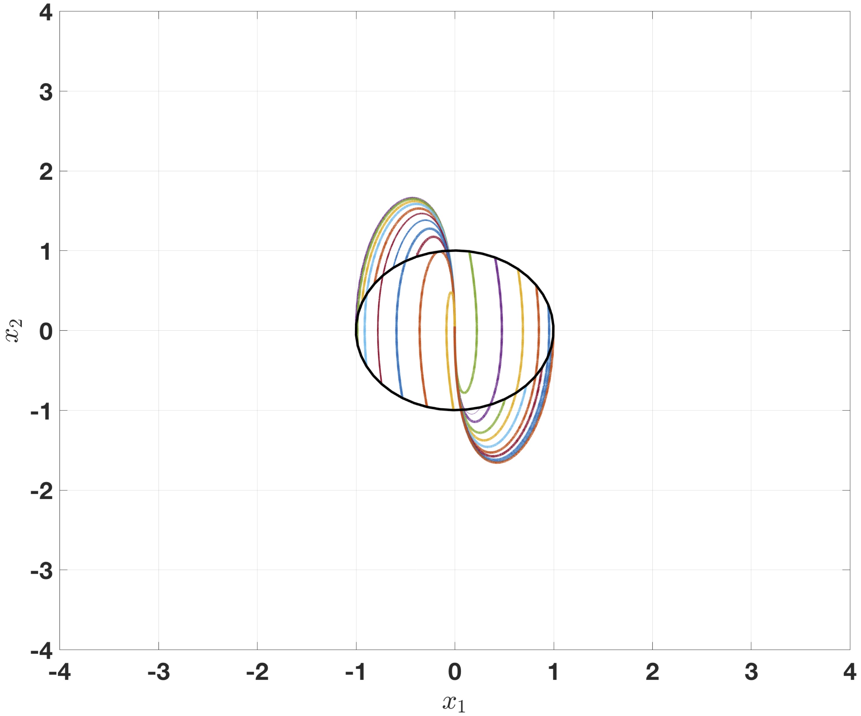
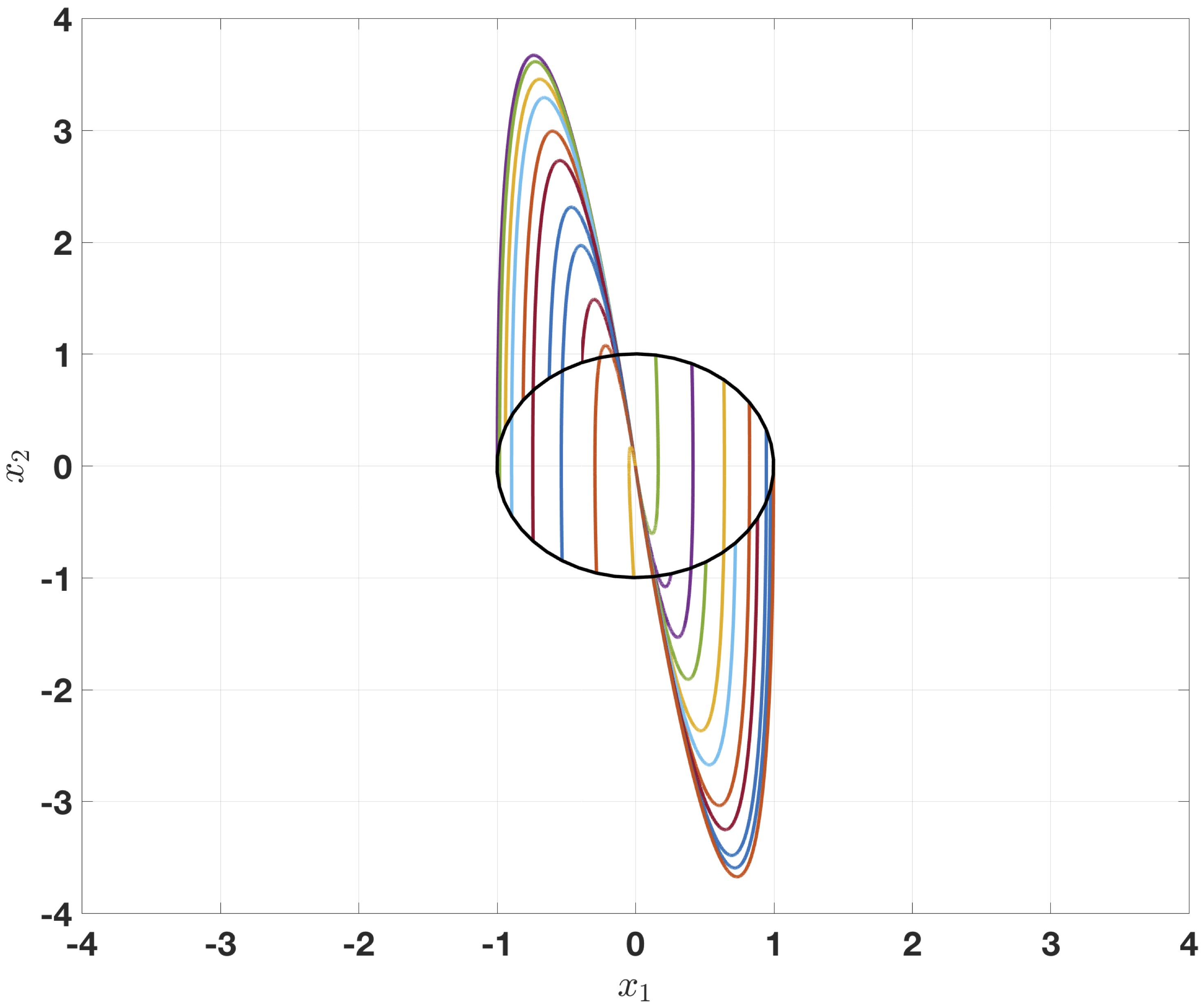
"Overshoots" of linear (left) and homogeneous (right) controllers ($n\!=\!2$, $\varepsilon=0.005$, $T\!=\!1$)Conclusion III
Homogeneous system may have smaller overshoot than linear one. - $\textbf{Linear control}:$ For any $\varepsilon>0$ and $T>0$ there
exists
$k=(k_1, k_2,..., k_n)$:
3 Generalized Homogeneity
3. 1 Linear Dilations
A $\textbf{linear continuous dilation}$ in $\mathbb{R } ^n$ is a matrix-valued function given by
$$\mathbf{ d } (s)=e^{sG_{\mathbf{ d } }}=\sum_{i=0}^{+\infty}\tfrac{s^iG_{\mathbf{ d } }^i}{i!}, \quad \quad s\in \mathbb{ R } $$
where $G_{\mathbf{ d } }\in \mathbb{ R } ^{n\times n}$ is an $\textit{anti-Hurwitz matrix}$ called a $\textbf{generator}$ of $\mathbf{ d } $.
Monotone dilation
Let $\|\cdot\|$ be a norm in $\mathbb{ R } ^n$ and $\mathbb{ R } $ be a $\textit{dilation}$ k in $\mathbb{ R } ^n$. A dilation $ \mathbf{d } $ is said to be strictly monotone with respect to $\|\cdot\|$ if $\exists \beta>0 : \|\mathbf{ d } (s)\|\leq e^{\beta s}$.
The standard dilation $\mathbf{d}(s)=e^{s}I_n$ is always monotone due to standard homogeneity (by definition) of any norm $\|e^s x\|=e^{s}\|x\|$.
Criterion of monotonicity of linear continuous dilation in $\mathbb{ R } ^n$
A linear continuous dilation $\mathbf{ d } $ is strictly monotone with respect to the weighted Euclidean norm
$\|x\|=\sqrt{x^{\top}Px}, \quad x\in \mathbb{ R } ^n,$where $0\prec P=P^{\top}\in \mathbb{ R } ^{n\times n}$, $\textbf{if and only if }$ the following linear matrix inequality holds $$ PG_{\mathbf{ d } }+G_{\mathbf{ d } }^{\top} P\succ 0, \quad \quad \quad \quad \quad \quad (3) $$ where $G_{\mathbf{ d } }\in \mathbb{ R } ^{n}$ is the generator of the dilation $\mathbf{ d } $. Moreover, one has $$ \!\begin{array}{c} \beta \|\mathbf{ d } (s)z\|^2\leq\frac{ \frac{d}{ds} \|\mathbf{ d } (s)z\|^2}2\leq \alpha \|\mathbf{ d } (s)z\|^2, \quad \forall s\in \mathbb{ R } , \forall z\in \mathbb{ R } ^n, \\ e^{\alpha s}\!\leq\!\lfloor \mathbf{ d } (s)\rfloor\!\leq\!\|\mathbf{ d } s)\|\!\leq e^{\beta s},\quad \forall s\!\leq\! 0, \quad \quad \quad \quad \quad \quad \quad \quad \quad (4) \\ e^{\beta s}\!\leq\!\lfloor \mathbf{ d } (s)\rfloor\!\leq\!\|\mathbf{ d } (s)\|\!\leq e^{\alpha s}, \quad \forall s\!\geq\! 0, \quad \quad \quad \quad \quad \quad \quad \quad \quad \end{array} $$ where $$\alpha=\frac{1}{2}\lambda_{\max}\left(P^{\frac{1}{2}} G_{\mathbf{ d } }P^{-\frac{1}{2}}+P^{-\frac{1}{2}}G^{\top}_{\mathbf{ d } } P^{\frac{1}{2}}\right)>0,$$ $$\beta=\frac{1}{2}\lambda_{\min}\left(P^{\frac{1}{2}} G_{\mathbf{ d } }P^{-\frac{1}{2}}+P^{-\frac{1}{2}}G^{\top}_{\mathbf{ d } } P^{\frac{1}{2}}\right)>0.$$
3. 2 Canonical Homogeneous Norm
Vector space
A vector space over the filed $\mathbb{ R } $ is a set $\mathbb{V}$ together with two operations:
satisfying certain axioms
- ${\color{blue}{vector \;\; addition\;\; }} \;\; \mathbb{V} \times \mathbb{V} \mapsto \mathbb{V}$ denoted by $ {\color{blue}{v+w}} $ for $v,w\in \mathbb{V}$.
- ${\color{red}{multiplication\;\; by\;\; a \;\; scalar\;\; } } \;\; \mathbb{ R } \!\times\!\mathbb{V} \mapsto \mathbb{V}$ denoted by $ {\color{red}{\alpha \cdot v}} $ for $\alpha\!\in\!\mathbb{ R } $, $v\!\in\!\mathbb{V}$.
- $\textit{Associativity}: u+(v +w)=(u+v)+w$
- $\textit{Distributivity}: (\alpha+\beta)u=\alpha\cdot u+\beta\cdot v$
- ...
For $\mathbb{V}=\mathbb{ R } ^n$ the multiplication of $v=(v_1,...,v_n)^{\top}\in \mathbb{ R } ^n$ by $\alpha\in \mathbb{ R } $ is traditionally defined as follows $\alpha v=(\alpha v_1,...,\alpha v_2)^{\top} \quad \quad {\color{red}{(standard\;\; dilation!!!)}}$
Question
$\textit{Is it possible to construct a vector space using a } $ $\underline{generalized \;\; dilation} $ $\textit{ as a multiplication by a scalar?} $
| $\textbf{Definition}$ (a norm): $\|\cdot\|\in C( \mathbb{ R }^n,\mathbb{ R }_+)$ is a norm if |
$\textbf{Definition} $ ( a homogeneous norm): $\|\cdot\|_{\mathbf{ d } }\!\in\!C(\mathbb{ R }^n,\mathbb{ R }_+\!)$ is a $\mathbf{ d } \text{-} $ homogeneous norm if |
| 1. $\|x\|=0 \Leftrightarrow x=\mathbf{ 0} $ | 1. $\|x\|_{\mathbf{ d } }=0 \Leftrightarrow x=\mathbf{ 0} $ |
| 2. $\|\pm e^{s}x\|=e^{s}\|x\|$ | 2. $\|\pm{\color{blue}{\mathbf{ d } (s)}}x\|_{\mathbf{ d } }=e^{s}\|x\| $ |
| 3. $\|x+y\|\leq \|x\|+\|y\|$ | $3.\|x{\color{blue}{\mathbf{ + }} } y\|_{\mathbf{ d } }\leq \|x\|_{\mathbf{ d } }+\|y\|_{\mathbf{ d } }$ |
Canonical homogeneous norm for monotone dilations
$\|x\|_{\mathbf{ d } }\!=\!e^{s_x} \quad \text{ where } \quad s_x\in \mathbb{ R }: \| \mathbf{ d } (-s_x)x\|\!=\!1 \quad x\neq\mathbf{ 0 } $
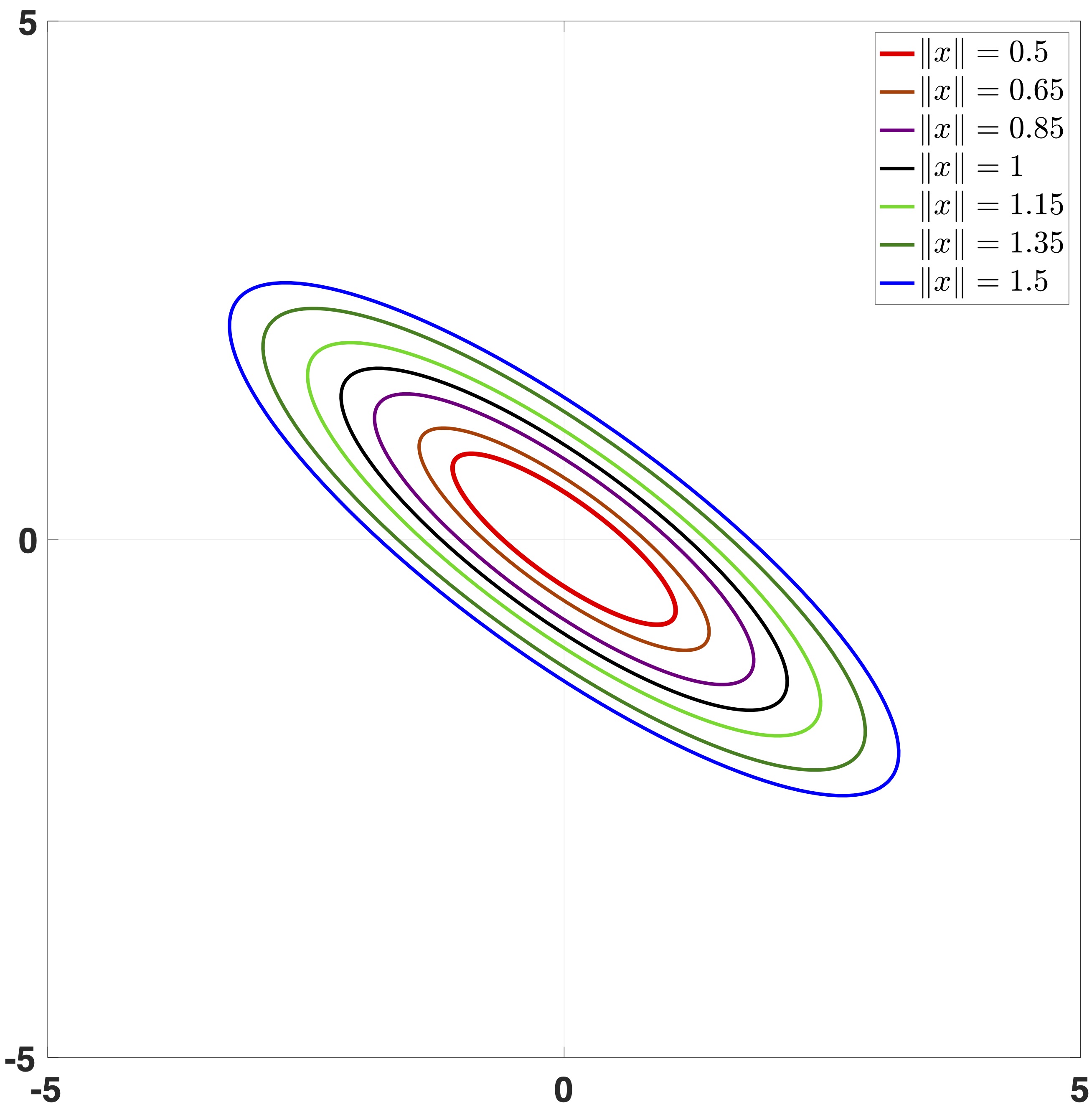 |
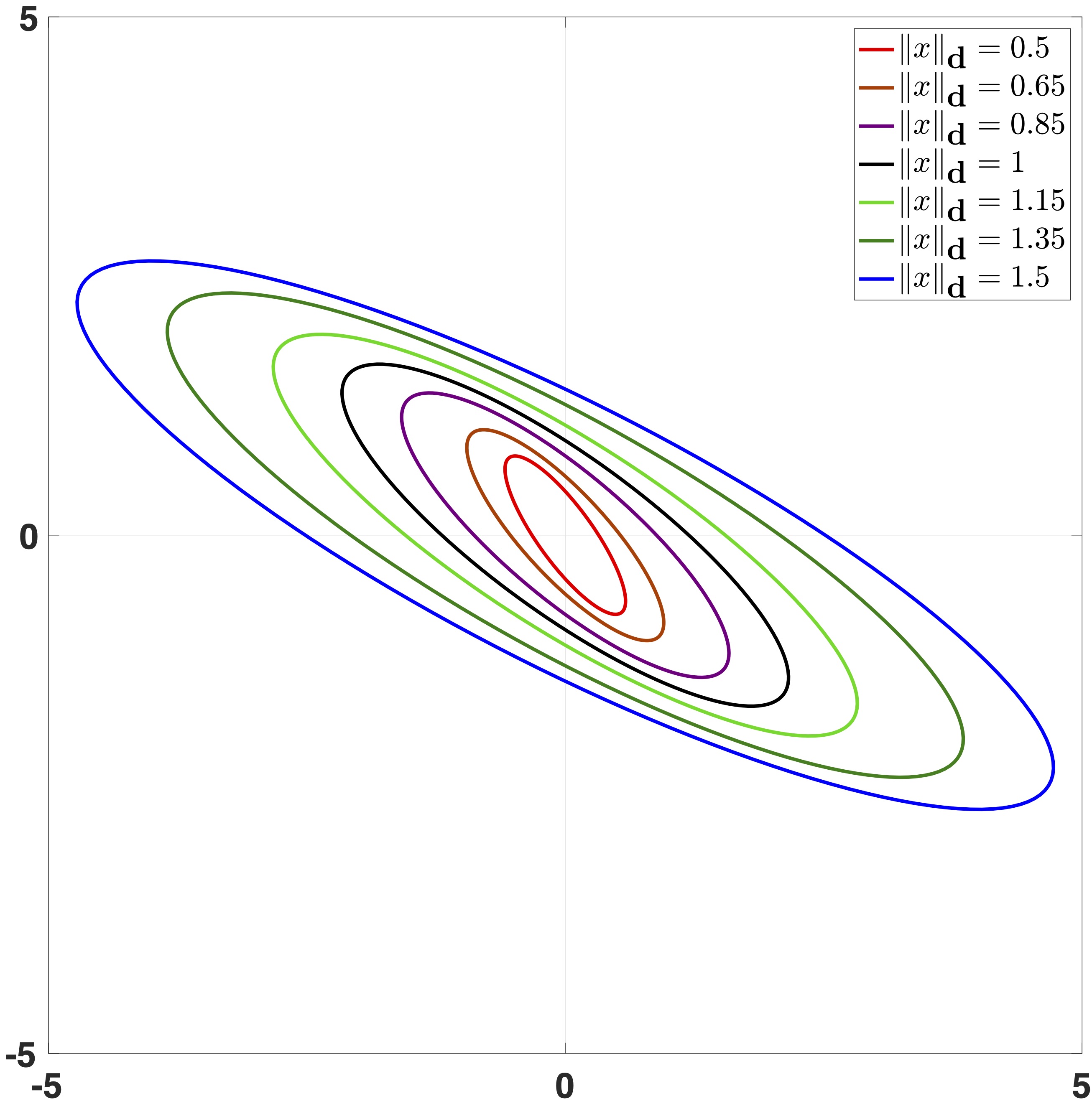 |
|
| $\|x\|=(0.5 x_1^2+0.4 x_1x_2+x_2^2)^{\frac{1}{2}}$ | $\|x\|_{\mathbf{ d } }$ induced by $\|x\|$ and $\mathbf{ d } (s)\!= \texttt{diag}\{e^{2s},e^s\}$ |
Level sets of the weighted Euclidean norm and the $\mathbf{ d }$-homogeneous norm.
Lemma $ ( $ Polyakov [ 14 ] $ ) $
If a linear continuous dilation $\mathbf{ d } $ in $\mathbb{ R } ^n$ is strictly monotone with respect to the norm $\|x\|=\sqrt{x^{\top} Px}, P\succ 0$ then
- $\|\cdot\|_{\mathbf{ d } } : \mathbb{ R } ^n\mapsto \mathbb{ R } _+$ is single-valued and $\|\cdot\|_{\mathbf{ d } }\in C^{\infty}(\mathbb{ R } ^n\backslash\{\mathbf{0} \})$;
- $\|x\|_{\mathbf{ d } }\to 0$ as $x\to \mathbf{ 0 } $ and $x\neq \mathbf{0} \Leftrightarrow \|x\|_{\mathbf{ d } }\neq \mathbf{ 0} $;
- $\|\pm \mathbf{ d } (s)x\|_{\mathbf{ d } }=e^{s}\|x\|_{\mathbf{ d } }$, $\forall s\in \mathbb{ R } , \forall x\in \mathbb{ R } ^n$;
- $\|x\|\!=\!1 \!\Leftrightarrow\! \|x\|_{\mathbf{ d } }\!=\!1$, $\|x\|\!<\!1\!\Leftrightarrow\! \|x\|_{\mathbf{ d } }\!<\!1$ and $\|x\|\!>\!1\! \Leftrightarrow\! \|x\|_{\mathbf{ d } }\!>\!1$;
- for $0<2\beta = \lambda_{\min}\left( PG_{\mathbf{ d } }+G_{\mathbf{ d } }^{\top}P \right)\leq \lambda_{\max}\left( PG_{\mathbf{ d } }+G_{\mathbf{ d } }^{\top}P \right)= 2\alpha$ one has $$ \left| \|x_1\|_{\mathbf{ d } }^{\alpha}-\|x_2\|_{\mathbf{ d } }^{\alpha}\right|\leq \|x_1-x_2\|, \quad \forall x_1,x_2\in B,\quad \quad \quad \quad \quad (5) $$ $$ \left| \|x_1\|_{\mathbf{ d } }^{\beta}-\|x_2\|_{\mathbf{ d } }^\beta\right|\leq \|x_1-x_2\|, \quad \forall x_1,x_2\in \mathbb{ R } ^n\backslash B,\quad \quad \quad (6) $$ where $B=\{x:\in\mathbb{ R } ^n: \|x\|\leq 1\}$ is the unit ball in $\mathbb{ R } ^n$.
- the derivative of $\|\cdot\|_{\mathbf{ d } }$ is given by $$ \frac{\partial \|x\|_{\mathbf{ d } }}{\partial x}=\|x\|_{\mathbf{ d } }\tfrac{x^{\top } \mathbb{ R } \mathbf{ d } ^{\top}(-\ln\|x\|_{\mathbf{ d } }) P \mathbf{ d } (-\ln\|x\|_{\mathbf{ d } })}{x^{\top } \mathbf{ d } ^{\top}(-\ln\|x\|_{\mathbf{ d } })PG_{\mathbf{ d } }\mathbf{ d } (-\ln\|x\|_{\mathbf{ d } })x}, \quad x\neq \mathbf{ 0} . \quad \quad \quad (7) $$
The canonical homogeneous norm introduces an alternative norm topology in $\mathbb{ R } ^n$.
Generalized homogeneous homeomorphism on $\mathbb{ R } ^n$
Let a linear continuous dilation $\mathbf{ d } $ be strictly monotone with respect to the norm $\|x\|=\sqrt{x^{\top} Px}$. The mapping $\Phi : \mathbb{ R } ^n \mapsto \mathbb{ R } ^n$ given by $$ \Phi(x)=\|x\|_{\mathbf{ d } } \mathbf{ d } (-\ln \|x\|_{\mathbf{ d } }) x, \quad x\in \mathbb{ R } ^n \quad \quad \quad (8) $$
is a homeomorphism in $\mathbb{ R } ^n$, its inverse has the form
$\Phi^{-1}(z)=\|z\|^{-1}\mathbf{ d } (\ln \|z\|)z, \quad z\in \mathbb{ R } ^n.$with $\Phi(\mathbf{ 0 } )=\Phi^{-1}(\mathbf{ 0 } )=\mathbf{ 0 } $ by continuity.
The following theorem justifies the name "norm" for the functional $\|\cdot\|_{\mathbf{ d } }$
Theorem ( Polyakov 2020 [ 15 ] )
Let a linear dilation $\mathbf{ d } $ be strictly monotone with respect to the norm $\|x\|=\sqrt{x^{\top} Px}$. Let an addition of vectors ${\color{blue}{ \mathbf{ + }}} : \mathbb{ R } ^n\times \mathbb{ R } ^n \mapsto \mathbb{ R } ^n$ and a multiplication by a scalar ${\color{blue}{\mathbf{ \cdot }}} : \mathbb{ R } \times \mathbb{ R } ^n\mapsto \mathbb{ R } ^n$ be defined as follows
- $x{\color{blue}{\mathbf{ + }}} y:=\Phi^{-1}(\Phi(x)+\Phi(y))$, where $x,y\in \mathbb{ R } ^n$,
- $\lambda{\color{blue}{ ∙}} x:= \texttt{sign}(\lambda)\mathbf{ d } (\ln |\lambda|)x$, where $\lambda\in \mathbb{ R } $, $x\in \mathbb{ R } ^n$.
Then the set $\mathbb{ R } ^n$ together with the operations ${\color{blue}{ \mathbf{ + }}}$ and ${\color{blue}{∙ }} $ is a linear vector space $\mathbb{ R } ^n_{\mathbf{ d } }$ with the norm $\|\cdot\|_{\mathbf{ d } }$.
4. Homogeneous Systems
4. 1 Homogeneous Mappings
Homogeneous function ( Kawsky [ 6 ] )
A $\underline{function }$ $h: \mathbb{ R }^n \mapsto \mathbb{ R }$ is said to be $\mathbf{ d } $-homogeneous of a degree $\nu\in \mathbb{ R }$ if
$$ h(\mathbf{ d } (s)x)=e^{\nu s}h(x) \quad \text{ for } \quad s\in\mathbb{ R }, \quad x\in \mathbb{ R }^n, \quad \quad \quad \quad \quad \quad (9) $$
where $\mathbf{ d } $ is a dilation in $\mathbb{ R }^n$.
Let $\mathcal{H}_{\mathbf{ d } }(\mathbb{ R }^n)$ be a set of all $\mathbf{ d } $-homogeneous functions $\mathbb{ R }^n \to \mathbb{ R }$ and $\deg_{\mathbf{ d } }(h) \in \mathbb{ R }$ denote the homogeneity degree of $h\in \mathcal{H}_{\mathbf{ d } }(\mathbb{ R }^n)$.
$\textit{Elements homogeneous arithmetics for functions } $ $ h,g \in \mathcal{H}_{\mathbf{ d } }(\mathbb{ R }^n):$- $\alpha h \in \mathcal{H}_{\mathbf{ d } }(\mathbb{ R }^n)$ and $\deg_{\mathbf{ d } }(\alpha h)=\deg_{\mathbf{ d } }(h)$ for any $\alpha\in \mathbb{ R }$;
- $h+g\in \mathcal{H}_{\mathbf{ d } }(\mathbb{ R }^n)$ provided that $\deg_{\mathbf{ d } }(h)=\deg_{\mathbf{ d } }(g)$;
- $h\cdot g\in \mathcal{H}_{\mathbf{ d } }(\mathbb{ R }^n)$ and $\deg_{\mathbf{ d } }(h\cdot g)=\deg_{\mathbf{ d } }(h)+\deg_{\mathbf{ d } }(g);$
- $\frac{h}{g}\!\in\! \mathcal{H}_{\mathbf{ d } }(\mathbb{ R }^n)$ and $\deg_{\mathbf{ d } }\left(\frac{h}{g}\right)=\deg_{\mathbf{ d } }(h)-\deg_{\mathbf{ d } }(g)$ if $g(x)\neq \mathbf{ 0 } $, $\forall x\in S$;
- if $h(x)=c$ for all $x \in \mathbb{ R }^n$ then $h\in \mathcal{H}_{\mathbf{ d } }(\mathbb{ R }^n)$ and $\deg_{\mathbf{ d } }(h)=0$ for $c\in \mathbb{ R }\backslash\{0\}$. If $c=0$ then $\deg_{\mathbf{ d } }(h)$ is any.
Properties of homogeneous functions ( Bhat & Bernstein [ 2 ] )
Let $h \in \mathcal{H}_{\mathbf{ d }}(\mathbb{ R } ^n)$ be such that $\sup_{x\in S} |h(x)|<+\infty$.
- If $\deg_{\mathbf{ d }}(h)>0$ then $h$ is bounded on any $\mathbf{ d }$-homogeneous ball $B_{\mathbf{ d }}(r)$ and
$h(x)\to 0$ as $x\to 0$
- If $\deg_{}(h)\!<\!0$ then $h$ is bounded on any set $\mathbb{ R } ^n\backslash B_{\mathbf{ d }}(r)$ with $r\!>\!0$ and
$h(x)\to 0$ as $x\to \infty $
- If $\deg_{\mathbf{ d }}(h) =0$ then $h$ is uniformly bounded on $\mathbb{ R } ^n$ and, moreover,
$h\equiv \textrm{const}$ provided that $h$ is continuous at zero.
$$ $$
Generalised homogeneous function theorem ( Polyakov 2020 [ 15 ] )
If $h \in \mathcal{H}_{\mathbf{ d }}(\mathbb{ R } ^n)$ is differentiable on $\mathbb{ R } ^n \backslash \{ \mathbf{ 0 } \}$ then
$$ \frac{\partial h(x)}{\partial x} G_{\mathbf{ d }}x=\deg_{\mathbf{ d }}(h) \cdot h(x), \quad \forall x\neq \mathbf{ 0 },n \quad \quad \quad (10) $$where $G_{\mathbf{ d }}\in \mathbb{ R } ^{n\times n}$ is a generator of the linear dilation $\mathbf{ d }$.
$$ $$
Homogeneous vector field ( Kawsky [ 6 ] )
A $\underline{vector \; field}$ $f:\mathbb{ R } ^n \!\mapsto\! \mathbb{ R } ^n$ is said to be $\mathbf{ d }$-homogeneous of degree $\mu\!\in\! \mathbb{ R } $ if
$$ f(\mathbf{ d }(s)x)=e^{\mu s}\mathbf{ d }(s)f(x) \quad \text{ for all } \quad s\in\mathbb{ R } , \quad u\in \mathbb{ R } ^n, \quad \quad \quad (11) $$
where $\mathbf{ d }$ is a dilation in $\mathbb{ R } ^n$.
Let $\mathcal{F}_{\mathbf{ d } }(\mathbb{ R } ^n)$ be a set of $\mathbf{ d } $-homogeneous vector fields $\mathbb{ R } ^n\mapsto \mathbb{ R } ^n$ and $\deg_{\mathbf{ d } }(f)$ denote the homogeneity degree.
$\textit{Elements homogeneous arithmetics for vector fields}:$
- If $h\in \mathcal{H}_{\mathbf{ d } }(\mathbb{ R } ^n)$ and $f\in \mathcal{F}_{\mathbf{ d } }(\mathbb{ R } ^n)$ then
$h\cdot f\in \mathcal{F}_{\mathbf{ d } }(\mathbb{ R } ^n) $ and $\deg_{\mathbf{ d } }(h\cdot f)=\deg_{\mathbf{ d } }(h)+\deg_{\mathbf{ d } }(f)$ - If $f_1,f_2 \in \mathcal{F}_{\mathbf{ d } }(\mathbb{ R } ^n)$ and $\deg_{\mathbf{ d } }(f_1)=\deg_{\mathbf{ d } }(f_2)$ then
$f_1\!+\!f_2\in \mathcal{F}_{\mathbf{ d } }(\mathbb{ R } ^n)$ and $\deg_{\mathbf{ d } }(f_1+f_2)=\deg_{\mathbf{ d } }(f_1)=\deg_{\mathbf{ d } }(f_2)$ - If $f_1,f_2\in \mathcal{F}_{\mathbf{ d } }(\mathbb{ R } ^n)$ then
$f_1(f_2)\in \mathcal{F}_{\mathbf{ d } }(\mathbb{ R } ^n)$
provided that $\deg_{\mathbf{ d } }(f_2)=0$ or $f_1$ is standard homogeneous.
$$ $$
Properties of homogeneous vector fields ( Polyakov 2020 [ 15 ] )
Let $f\in \mathcal{F}_{\mathbf{ d } }(\mathbb{ R } ^n)$ be such that $M:=\sup_{x\in S}\|f(x)\|<+\infty$
where $\alpha=\lambda_{\max}\left(P^{1/2}G_{\mathbf{ d } }P^{-1/2}+P^{-1/2}G_{\mathbf{ d } }P^{1/2}\right)$ and $\beta=\lambda_{\min}\left(P^{1/2}G_{\mathbf{ d } }P^{-1/2}+P^{-1/2}G_{\mathbf{ d } }P^{1/2}\right)$.
- If $\deg_{\mathbf{ d } }(f)+\beta>0$ then $f$ is bounded on $B_{\mathbf{ d } }(r)$ and $\|f(x)\|\to 0$ as $\|x\|\to 0$
- f $\deg_{\mathbf{ d } }(f)+\alpha<0$ then $f$ is bounded on $\mathbb{ R } ^{n}\backslash B_{\mathbf{ d } }(r)$ and $\|f(x)\|\to 0$ as $\|x\|\to +\infty$
- If $\deg_{\mathbf{ d } }(f)+\beta=\deg_{\mathbf{ d } }(f)+\alpha=0$ then $f$ is uniformly bounded on $\mathbb{ R } ^{n}$,
$$ $$
Generalised theorem for vector fields ( Polyakov 2020 [ 15 ] )
If $f\in \mathcal{F}_{\mathbf{ d } }(\mathbb{ R } ^n)$ is differentiable on $\mathbb{ R } ^n\backslash\{\mathbf{0} \}$ then
$$ \label{eq:hom_op_deriv_relation_Rn} \frac{\partial f(x)}{\partial x} G_{\mathbf{ d } }x=(\deg_{\mathbf{ d } }(f) I_n+G_{\mathbf{ d } })f(x) \text{ for all } x\in \mathbb{ R } ^n\backslash\{\ \mathbf{ 0 } \}. \quad \quad \quad (12) $$
$$ $$
On linear homogeneous vector fields (Polyakov 2020, Zimenko et al. 2020)
The following three claims are equivalent ( [ 15 ] , [ 20 ] ) :
- a vector field $x\mapsto Ax$ with $x\in \mathbb{ R } ^n$ and $A\in \mathbb{ R } ^{n\times n}$ is $\mathbf{ d } $-homogeneous of degree $\mu\neq 0$ with respect to a linear continuous dilation $\mathbf{ d } $ in $\mathbb{ R } ^n$.
- there exists an anti-Hurwitz matrix $G_{\mathbf{ d } }\in \mathbb{ R } ^{n\times n}$ such that $ \begin{equation}\label AG_{\mathbf{ d } }=(\mu I+G_{\mathbf{ d } })A; \quad \quad \quad (13) \end{equation} $
- the matrix $A$ is nipotent.
$\textbf{Conclusion}: $
- $A^n\neq \mathbf{ 0 } \Rightarrow G_{\mathbf{ d } }=I_n$, $\mu=0$
- $A^n=\mathbf{ 0 } \Rightarrow \forall \mu\neq \mathbf{0 } $, $\exists G_{\mathbf{ d } } - anti-Hurwitz$ : $AG_{\mathbf{ d } }=(\mu I_n+G_{\mathbf{ d } })A$
How to find $G_{\mathbf{ d } }$ for a given $\mu\neq 0$?
$\textbf{A possible solution:} $
- find $G_0$ such that $AG_{0}=(I_n+G_{0})A$ (i.e., solve the linear equation)
- take $G_{\mathbf{ d } }\!=\!\epsilon I_n\!+\!\mu G_{0}$ with a large enough $\epsilon\!>0$ (to make $G_{\mathbf{ d } }$ anti-Hurwitz)
$$ $$
Local Homogeneity (Andrieu et al 2008 [1] )
$$ $$
A $\mathbf{ d } $-homogeneous vector field $f_{L} : \mathbb{ R } ^n \mapsto \mathbb{ R } ^n$ of degree $\nu\in \mathbb{ R } $ is said be $\mathbf{ d } $-homogeneous approximation of $f$ at $L$-limit (with $L=0$ or $L=\infty$) if
$$\lim_{r\to L^+} \sup_{x\in S } \|r^{-\nu}\mathbf{ d } (-\ln r)f(\mathbf{ d } (\ln r)x)-f_L(x)\|=0, $$
where $S=\{x:\in \mathbb{ R } ^n: \|x\|=1\}$ is the unit sphere in $\mathbb{ R } $.
$$ $$
$\textbf{Example:} \;\;\; $If $ f(x)= -x^3+x^4-x^5 $then
- the linearization at zero gives $\left.\frac{\partial f(z)}{\partial z}\right|_{z=0} x=\left.3z^2\right|_{z=0} x=0$
- the homogeneous approximation at zero gives $f_0(x)=-x^3$.
4. 2 Homogeneous Differential Equations
Any linear system
$$ \dot x=Ax, \quad t\in \mathbb{ R }, \quad x(t)\in \mathbb{ R }^n, \quad A\in \mathbb{ R }^{n\times n}, \quad x(0)=x_0 $$
is standard homogeneous and its solution $x(t,x_0)=e^{tA}x_0$ is symmetric with respect to the scaling of the initial condition $x(t,e^sx_0)=e^sx(t,x_0)$
$$ $$
Symmetry of a flow of generalized homogeneous linear vector field
$$ $$
Let $\mathbf{ d } $ be a linear dilation and let a linear vector field $f:\mathbb{ R }^n\mapsto \mathbb{ R }^n$ given by
$$ f(x)=Ax, \quad x\in \mathbb{ R }^n, \quad A\in \mathbb{ R }^{n\times n}$$be $\mathbf{ d } $-homogeneous of degree $\mu\in\mathbb{ R }^n$ (i.e., $A\mathbf{ d } (s)=e^{\mu s}\mathbf{ d } (s)A$) then
$$ e^{tA}\mathbf{ d } (s)=\mathbf{ d } (s)e^{tAe^{\mu s}}, \quad \forall s\in \mathbb{ R }, \quad \forall t\in \mathbb{ R }. $$
Let $x(t,x_0)$ denote a solution of the system
$$ \dot x(t)=f(x(t)), \quad t>0, \quad \quad \quad (14) $$with the initial condition $x(0)=x_0\in \mathbb{ R }^n$.
$$ $$
Theorem (Zubov 1958 , Kawsky 1991 )
$$ $$
Let $\mathbf{ d } $ be a dilation in $\mathbb{ R }^n$ and the vector field $f$ be $\mathbf{ d } $-homogeneous of degree $\mu\in \mathbb{ R }$. If $x(t,x_0)$ with $t\in [0, T]$ is a solution of the system (14) with the initial condition $x(0)=x_0$ then, for any $s\in \mathbb{ R }$,
$$ x(t,\mathbf{ d } (s)x_0)=\mathbf{ d } (s)x(e^{\mu s}t,x_0), \quad t\in [0, e^{-\mu s}T]$$
is a solution of (14) with the $ \underline{scaled} $ initial condition $x(0)=\mathbf{ d } (s)x_0$.
$$ $$
Corollary
Let $f$ be a continuous $\mathbf{ d } $-homogeneous vector field of degree $\mu\leq 0$ then the system $\dot x=f(x)$ is $complete . $
$$ $$
Lyapunov Stability (Lyapunov 1892)
The system (14) is said to be locally (globally) uniformly $\textit{Lyapunov stable}$ if , $\exists \varepsilon\in \mathcal{K}$
$$ |x(t,x_0)|\leq \varepsilon(|x_0|), \quad \forall t\geq 0, \quad \forall x_0\in \Omega,$$
where $\Omega$ is a neighborhood of the origin (resp., $\Omega=\mathbb{R}^n$)
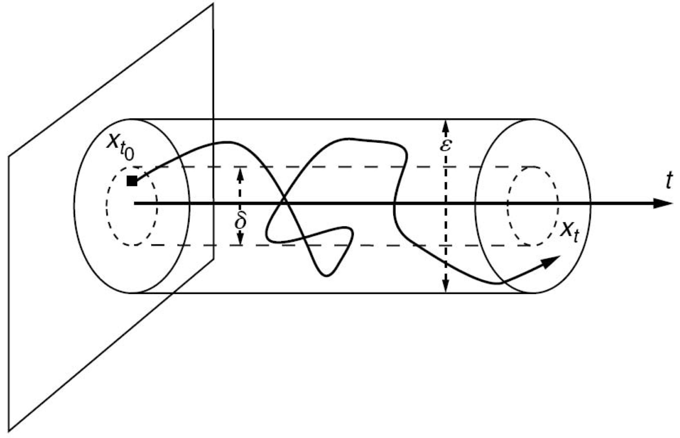
Illustration of Lyapunov stability
Proposition (Bhat & Bernstein 2005 [2] )
Let $f:\mathbb{ R} ^n\mapsto\mathbb{ R }^n$ be a continuous $\mathbf{ d } $-homogeneous vector field. The system (14) is Lyapunov stable if and only if it has a positively invariant, bounded neighborhood of the origin.
$$ $$
Asymptotic Stability (Lyapunov 1892)
The system (14) is said to be locally (globally) uniformly $\textit{asymptotically stable}$ ${\color{red}{observer}}$ if $\exists \beta\in \mathcal{KL}$
$$ \|x(t,x_0)\|\leq \beta(|x_0|,t), \quad \forall t\geq 0, \quad \forall x_0\in \Omega,$$
where $\Omega$ is a neighborhood of the origin (resp., $\Omega=\mathbb{ R} ^n$)
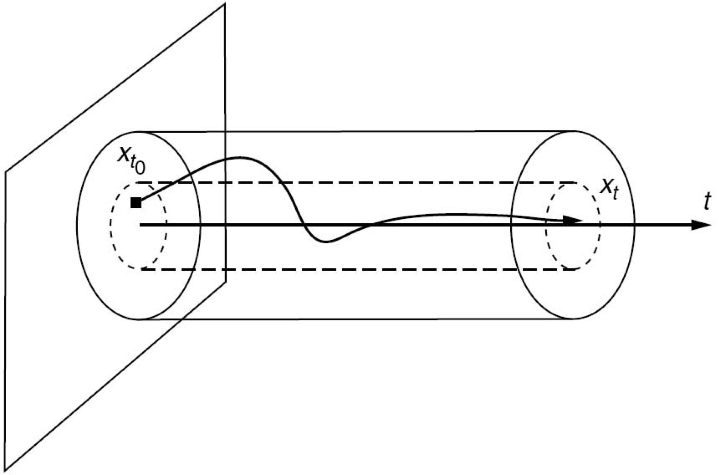
Illustration of asymptotic stability
Let a continuous vector field $f:\mathbb{ R } ^n\mapsto \mathbb{ R } ^n$ be $\mathbf{ d } $-homogeneous of degree $\mu$. Let $m>0$ be an arbitrary positive number.
The system (14) is asymptotically stable if and only if there exists a positive definite homogeneous function $V\in C(\mathbb{ R } ^n)\cap C^{\infty}(\mathbb{ R } ^n\backslash\mathbf{ 0 } )$ of degree $m$:
$$ \dot V(x)\leq -\rho V^{1+\frac{\mu}{m}}(x), \quad \forall x\in \mathbb{ R } ^n\backslash\{\mathbf{ 0 } \}, \quad \quad \quad (15) $$
where $\rho>0$ is some number.
$$ $$
Corollary (Nakamura et al 2002 [9] )
Let $f$ be $\mathbf{ d } $-homogeneous of degree $\mu \!\in\! \mathbb{ R } $. If (14 ) is locally asymptotically stable then it is
- globally uniformly $\textbf{finite-time stable}$ for $\mu<0$ with a settling-time function $T$ being continuous at $x=0$;
- globally $\textbf{nearly fixed-time stable}$ for $\mu>0$, i.e.,
$\forall r>0, \exists T_r>0 \text{ such that } \|x(t,x_0)\|\leq r, \forall t\geq T_r, \forall x_0\in \mathbb{ R } ^n.$
$$ $$
Let us consider the perturbed nonlinear system:
$$ \dot x=f(x,q), \quad t>0, \quad x(t)\in \mathbb{ R } ^n, \quad q(t)\in \mathbb{ R } ^{k}, \quad x(0)=x_0 \quad \quad \quad (16) $$
Definition (Sontag 1989 [22] )
A system (16) is said to be Input-to-State Stable (ISS) with respect to $q\in L^{\infty}(\mathbb{ R } ,\mathbb{ R } ^{k})$ if there exist $\beta\in \mathcal{KL}$ and $\gamma \in \mathcal{K}$ such that
$$ \|x(t)\|\leq \beta(\|x_0\|,t)+\gamma(\|q\|_{L^{\infty}((t_0,t),\mathbb{ R } ^k)}). \quad \quad \quad (17) $$
$$ $$
Let $\mathbf{ d } _q$ be a dilation in $\mathbb{ R } ^n$ and $\mathbf{ d } _q$ be a dilation in $\mathbb{ R } ^m$ such that $\exists \mu\in \mathbb{ R } :$
$$f(\mathbf{ d } _x(s)x,\mathbf{ d } _q(s)q)=e^{\mu s}\mathbf{ d } _x(s)f(x,q) \quad \forall x\in \mathbb{ R } ^m, \forall q\in \mathbb{ R } ^m, \forall s\in \mathbb{ R } .$$
If the system $\dot x=f(x,\mathbf{0 } )$ is asymptotically stable then the system (16) is ISS.
$$ $$ $$ $$
4. 3 Homogeneous Control Design
Let us consider the control system $$ \dot x=Ax+ Bu, \quad t>0, \quad \quad \quad (18) $$
where $x\in \mathbb{ R } ^n$ - system state, $u\in \mathbb{ R } ^m$ - control input, $A\in \mathbb{ R } ^{n\times n}, B\in \mathbb{ R } ^{n\times m}$.
$$ $$
The Problem of Homogeneous Stabilization
$$ $$
Given $\mu\in \mathbb{ R } $ the control aim is to design a dilation $\mathbf{ d } $ in $\mathbb{ R } ^n$ and a feedback control $u:\mathbb{ R } ^n\mapsto \mathbb{ R } ^m$ such that the closed-loop system is
- $\mathbf{ d } $-homogeneous of degree $\mu$, i.e., for $f(x)=Ax+Bu(x)$ one holds
$$f(\mathbf{ d } (s)x)=e^{\mu s}\mathbf{ d } (s)f(x), \quad \forall x\in \mathbb{ R } ^n, \quad \forall s\in \mathbb{ R } ;$$
- asymptotically stable ($\Rightarrow$ finite-time stability for $\mu<0$).
$$ $$
$$ $$
The system (18) is homogeneously stabilizable with $\mu\neq 0$ $\textbf{if and only if } $ the pair $\{A,B\}$ is controllable . For any controllable pair $\{A, B\}$ one holds
- the linear algebraic equation $$ AG_0-G_0A+BY_0=A, \quad G_0B=\mathbf{ 0} \quad \quad \quad (19) $$
has a solution $Y_0\in\mathbb{ R } ^{m\times n}$, $G_0\in \mathbb{R}^{n\times n}$ and for any solution one hold
the matrix $G_0-I_n$ is invertible is invertible;
- $G_{\mathbf{d}}\!=\!I_n\!+\!\mu G_0$ is anti-Hurwitz for $\mu\!\leq 1/ n^*$, where $n^*\!\in\! \mathbb{N}$ is a minimal number such that $ \texttt{rank}[B,AB,...,A^{n^*-1}B]=n$;
- the matrix $\!A_0\!=\!A+BK_0$ is nilpotent,$K_{0}\!=\!Y_0(G_0-I_n)^{-1}\!$ and $ \!A_0G_{\mathbf{d}}\!=\!(G_{\mathbf{d}}\!+\!\mu I_n)A_0,\! G_{\mathbf{d}}B\!=\!B; $ (20)
- the linear algebraic system
$$ \begin{array}{c} A_0X\!+\!XA_0^{\top}\!\!+\!BY\!+\!Y^{\top}\!B^{\top}\!\!+\!\rho(G_{\mathbf{ d } }X\!+\!XG_{\mathbf{ d } }^{\top})\!=\!\mathbf{ 0 } , \\ G_{\mathbf{ d } }X\!+\!XG_{\mathbf{ d } }^{\top}\!\succ\! 0, \quad X\!=\!X^{\top}\!\succ\! 0 \end{array} \quad \quad \quad (21) $$
has a solution $X\!\in\! \mathbb{R}^{n\times n}$, $Y\!\in\! \mathbb{R}^{m\times n}$ for any $\rho\!\in\! \mathbb{ R } _+$;
the homogeneous norm $\|\cdot\|_{\mathbf{d}}$ induced by $\|x\|=\sqrt{x^{\top} X^{-1}x}$ is a Lyapunov function of the system (18) with the feedback law
$$ u(x)\!=\!K_0x+\|x\|_{\mathbf{d}}^{1+\mu}K\mathbf{d}(-\ln \|x\|_{\mathbf{d}})x, \quad K\!=\!YX^{-1}, \quad \quad \quad (22) $$where $\mathbf{d}$ is a dilation generated by $G_{\mathbf{d}}$; moreover,
$$ \tfrac{d}{dt} \|x\|_{\mathbf{d}} = -\rho \|x\|^{1+\mu}_{\mathbf{d}}, \quad x\neq \mathbf{0}; \quad \quad \quad (23) $$
- $u \in C^{\infty}(\mathbb{ R } ^{n}\backslash\{\mathbf{ 0 } \})$ and $|u(x)| \leq K_0|x| +\lambda_{\max}(X)\|x\|_{\mathbf{ d } }^{1+\mu}, \forall x\in \mathbb{ R } ^n$, $\forall \mu\geq -1$;
- the system (18), (22) is $\mathbf{ d } $-homogeneous of degree $\mu$.
$$ $$
4. 4 Homogeneous Observer Design
Let us consider the system
$$ \dot x=Ax+p(t), \quad t>0, \quad y=Cx \quad \quad \quad (24) $$
where $x\in \mathbb{ R } ^n$ - $ ({\color{red}{unknown}})$ system state, $p(t)\in \mathbb{ R } ^n$ - known exogenous input, $y\in \mathbb{ R } ^k$ - measured system output, $A\in \mathbb{ R } ^{n\times n}$ and $C\in \mathbb{ R } ^{k\times n}$.
$$ $$
The Problem of Homogeneous Observer Design
Given $\mu\in \mathbb{ R } $ we need to design a dilation $\mathbf{ d } $ in $\mathbb{ R } ^n$ and an observer:
$$ \dot z=Az+p+g(Cz-y), \quad z(0)=\mathbf{ 0 } \quad g: \mathbb{ R } ^{k}\mapsto \mathbb{ R } ^n $$
such that the error equation
$$ \dot \epsilon=A\epsilon+g(C\epsilon), \quad \epsilon=z-x $$
is $\mathbf{ d } $-homogeneous of degree $\mu$, i.e., for $f(\epsilon)=A\epsilon+g(C\epsilon)$ one holds $$ f(\mathbf{ d } (s)\epsilon)=e^{\mu s}\mathbf{ d } (s)f(\epsilon), \quad \forall \epsilon\in \mathbb{ R } ^n, \quad \forall s\in \mathbb{ R } ;$$
s asymptotically stable.
$$ $$
$$ $$
The system (24) is homogeneously observable with degree $\mu \neq 0$ $\textbf{if and only if} $ the pair $\{A,C\}$ is observable. For any observable pair $\{A,C\}$ one holds
- the linear algebraic equation
$$ AG_0-G_0A+Y_0C=A, \quad CG_0=\mathbf{0} \quad \quad \quad (25) $$
has a solution $Y_0\in \mathbb{R}^{n\times k}$, $G_0\in \mathbb{R}^{n\times n}$ and for any solution one holds
- the matrix $G_0+I_n$ is invertible
- the matrix $G_{\mathbf{d}}=I_n+\nu G_0$ is anti-Hurwitz for $\nu\geq -1/\tilde n$, where $\tilde n$ is a minimal natural number such that
$ \texttt{rank}\left[\begin{smallmatrix}C\\CA\\...\\CA^{n-1}\end{smallmatrix}\right]=n.$
- the matrix $A_0=A+L_0C$ is nilpotent, $L_0=-(G_{0}+I_n)^{-1}Y_0$ and
$ A_0G_{\mathbf{d}}=(\nu I_n +G_{\mathbf{d}})A_0, \quad CG_{\mathbf{d}}=C; $
- the algebraic system $$ \! \!\!\!\!\!\! \begin{array}{c} PA_0\!+\!A_0^{\top}\!P\!+\!YC\!+\!C^{\top}\!Y^{\top}\!\!+\!\rho(PG_{\mathbf{d}}\!+\!G_{\mathbf{d}}^{\top}P)\!=\!\mathbf{ 0 } , \\ PG_{\mathbf{d}}+G_{\mathbf{d}}^{\top}P\succ 0, \quad P=P^{\top}\succ 0 \end{array} \quad \quad \quad (26) \!\!\!\!\!\! $$ has a solution $P\in \mathbb{ R } ^{n\times n}$, $Y\in \mathbb{ R } ^{k\times n}$ for any $\rho\in \mathbb{ R } _+$.
- the canonical homogeneous norm $\|\epsilon\|_{\mathbf{ d } }$ induced by the weighted Euclidean norm $\|\epsilon\|=\sqrt{\epsilon^{\top}P\epsilon}$ is a Lyapunov function (at least if $\nu$ close to $0$) for the error equation (28) of the observer $$ \dot z\!=\!Az\!+\!p\!+\!\left( L_0\!+ {\color{blue}{\!{ {|Cz\!-\!y|^{\nu-1}\mathbf{ d } (\ln |Cz-y|)}} } } L\right)(Cz\!-\!y), \quad z(0)\!=\!\mathbf{ 0 } , \quad \quad \quad (27) $$ where $L=P^{-1}Y$;
- the error equation $$ \dot \epsilon=(A_0+|C\epsilon|^{\nu-1}\mathbf{ d} (\ln |C\epsilon|)LC)\epsilon, \quad \epsilon=z-x \quad \quad \quad (28) $$ is continuous for $\nu>-1/n^*$ and discontinuous for $\nu=-1/n^*$;
- the error system (27) is $\mathbf{ d } $-homogeneous of degree $\nu$,
$\textbf{Remarks}$
- without loss of generality, the identity $=0$ in the system of LMIs (21) (resp. (26)) can replaced with inequality $\preceq 0$;
- combing the homogeneous controllers/observers with positive and negative degrees, a locally homogeneous $\textbf{fixed-time stable}$ system can be designed: $$\exists T_{\max}>0\quad : \quad x(t,x_0)=\mathbf{0 } , \quad \forall t\geq T_{\max}, \quad \forall x_0\in \mathbb{ R } ^n$$
$$(\text{resp., } \exists T_{\max}>0\quad : \quad z(t)=x(t,x_0), \quad \forall t\geq T_{\max}, \quad \forall x_0\in \mathbb{ R } ^n)$$
5. On Discretization of Homogeneous Systems
5. 1 Control Discretization
Due to a digital implementation of controller one holds
$$u(t)=u_j, \quad \forall t\in [t_j,t_{j+1}), j=0,1,2,...$$
where $t_{j+1}-t_j\geq h>0$, $t_0=0$.
Moreover, the measurements are samples as well. Let us assume (for simplicity) that the measurements and control samplings are synchronized, i.e., at time $t=t_j$ we can measure $x_j=x(t_j)$. Several algorithms of digital implementation of homogeneous controller can be suggested in this case .
$$ $$Explicit discretization of homogeneous control
$$u_j=K_0x_j+\|x_j\|^{1+\mu}_{\mathbf{ d } } K\mathbf{ d } (-\ln \|x_j\|_\mathbf{ d } )x_j$$
$$ $$
Using the so-called semi implicit Euler method the closed-loop system can be approximated as follows
$x(t_{j+1})\approx z_{j+1}=x_j+h(A+BK_j)z_{j+1}, \quad K_j=K_0+\|x_j\|_\mathbf{ d }^{1+\mu} K\mathbf{ d } (-\ln \|x_j\|_\mathbf{ d } )$
Hence, $z_{j+1}=(I_n-h(A+BK_j )^{-1}x_j$ the semi-implicit control discritization can be defined as follows.
$$ $$
Semi-implicit discretization of homogeneous control
$$ u_j=K_j(I_n-(t_{j+1}-t_j)(A+BK_j ))^{-1}x_j, \quad K_j=K_0+\|x_j\|^{1+\mu}_{\mathbf{ d } } K\mathbf{ d } (-\ln \|x_j\|_\mathbf{ d } )$$
$$ $$
5. 2 Observer Discretization
To implement a homogeneous observer in a digital device the system (27) has to be properly discretized under assumption that the output measurements $y$ and the exogenous input $p$ are sampled:
$$y(t)=y(t_j), \quad p(t)=p(t_j), \quad t\in [t_j,t_{j+1}), j=0,1,2,...$$
where $t_{j+1}-t_{j}\geq h>0$. The observer's discretizations are defined using the same ideas as controllers discretization.
$$ $$
Explicit discretization of homogeneous observer
$$ z_{j+1}=z_j+(t_{j+1-t_j})\left(Az_j\!+\!p_j\!+\!(L_0\!+\!|Cz_j\!-\!y_j|^{\nu-1} \mathbf{d}(\ln |Cz_j\!-\!y_j|)L)(Cz_j\!-\!y_j)\right)$$
where $z_0=z(0)$ and $z_j\approx z(t_j)$. The semi-implicit Euler's method gives
$$ z_{j+1}=z_j+h\left(Az_{j+1}+p_j+(L_0+|Cz_j-y_j|^{\nu-1} \mathbf{d}(\ln |Cz_j-y_j|)L(Cz_{j+1}-y_j)\right)$$
Semi-implicit discretization of homogeneous observer
$$z_{j+1}=Q_j^{-1}\left(z_j+(t_{j+1}-t_j)\left(p_j-L_j y_j\right)\right)$$
where $Q_j=I_n-h(A+L_jC)$ and
$$L_j=L_0+|Cz_j-y_j|^{\nu-1} \mathbf{d}(\ln |Cz_j-y_j|)L.$$
The presented discretizations have different computational complexity and can be selected for practical implementation dependently of the available computational resources.
6 Theoretical conclusions
-
Homogeneous systems may have faster convergence, better robustness and smaller overshoots than linear systems.
-
Theorems 1 and 2 are constructive and provide a way to define parameters of homogeneous controllers/ observer by solving certain algebraic systems. All functions of controllers and observers design are developed in HCS Toolbox based on the mentioned theorems and their corollaries.
-
In the view of the structure of the homogeneous controllers/observers many existing linear controllers/observers can be easily upgraded/transformed to homogeneous ones.