Homogeneous Curves
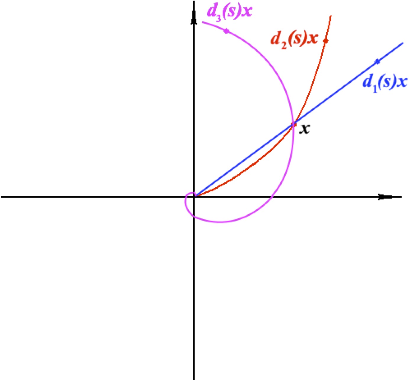
Given $x\in \mathbb{ R } ^n$ the set
$\begin{equation} \Gamma_{\mathbf{ d } }(x)=\{\mathbf{ d } (s)x : s\in \mathbb{ R } \}, \end{equation}$
is called a $\mathbf{ d } $-{homogeneous curve}.
Design of a homogeneous curve
The function ${\color{red} { \texttt{hcurve }} } $ generates an array of points on the homogeneous curve crossing the point $x\in\mathbb{ R } ^n$.
- $\textbf{Input parameters}: {\color{blue}x}, {\color{blue}{G_{\mathbf{ d } }}}, {\color{blue}{s_l}}$ (array of points $s_i\in \mathbb{ R } ,i=1,2,...$)
- $\textbf{Output parameters}: {\color{magenta}{x_l}} $ (array of points corresponding to $s_l$)
${\color{red} { \texttt{demo_hcurve.m}} } $
%%%%%%%%%%%%%%%%%%%%%%%%%%%%%%%%%%%%%%%%%%%%%%%%%%%%%%%%%%%%%%%%%%%%%%%%%%% %% %% Plot of homogeneous curve %% %%%%%%%%%%%%%%%%%%%%%%%%%%%%%%%%%%%%%%%%%%%%%%%%%%%%%%%%%%%%%%%%%%%%%%%%%%% Gd=[2 0; 1 1]; % a dilation in R^2 %plotting homgoeneous curves figure1 = figure; axes1 = axes('Parent',figure1); hold(axes1,'on'); sl=[-5:0.01:2]; N=5; %number of curves to plot for i=0:N x=[cos(2*pi*i/N);sin(2*pi*i/N)]; % vector x in R^2 zl=hcurve(x,Gd,sl); plot(zl(1,:),zl(2,:),'LineWidth',2); end; xlabel('$x_1$','Interpreter','latex'); ylabel('$x_2$','Interpreter','latex'); xlim(axes1,[-8 8]); ylim(axes1,[-2 2]); box(axes1,'on'); set(axes1,'FontSize',30,'XGrid','on','XTick',[-5 0 5],'YGrid','on','YTick',... [-2 -1 0 1 2]);