BioComputing's Network-Graph Tool

BioComputing team, Inria Lille and Université de Lille, France

Joachim Niehren and Cristian Versari

Version 1.99 from 30 Aug 2023, @Copyright August 2016

Why the Network-Graph tool?

Purpose

The main purpose of BioComputing's Network-Graph tool is to draw the graphs of reaction networks. If not given, the x-y-coordinates of all species and reactions in the network are computed with graphviz. An appropriate XML syntax for specifying reaction networks with partially known kinetics is provided by an XML schema. It is defined by a document type descriptor (DTD) for defining the hierachical structure and a Schematron schema for imposing the coherence of the data values. The tool can solve the following tasks: The BioComputing's Network-Graph tool is a module of a larger tool that was developed for illustrating reaction networks graphically in the context a series of research articles including:

Example Graph for Control of Ilv-Leu Promoter

An example graph generated for the PIlv-Leu network is given below. It has partial kinetic information only. There are four actors, which represent the protein binding sides BSCodY, BSCcpA, BSTnrA and the promoter PIlv-Leu of the metabolites isoleucine Ilv and leucine Leu. Of those two, only the metabolite Leu is in the network. The dashed arrow starting at the Leu node means that Leu has an outflow to the context. There are also two inflows from the context, which produce the proteins CodY and TnrA. Reaction 2 has PIlv-Leu as its product, meaning that it activates the Ilv-Leu promoter. Note that 2 has an implicit degradation reaction, which is indicated by the squirreled arrow. It also has three inhibitors, BSCodY, Leu, and BSTnrA, and one accelerator BSCcpA. Reaction 1 has CodY as activator. CodY has an inflow and an explicit degradation reaction 51. The four reactions in orange 1, 14, 7, and 8 are knockout candidates. Protein CcpA is essential, which is indicated by the red border, so no knockout may block the production of CcpA. The colored arrows on the product and reactant edges can be used to indacte the fluxes computed by a elementary mode based flux analysis. PIlv-Leu network

Example Graph for SBML Model B111

This an example for a reaction network with complete kinetic information. It was compiled to BioComputing reaction network format from the SBML model B111 of curated part of the BioModels database, via Core SBML. Note that this compiler is not provided within the present graph drawing tool for reaction networks in BioComputing's format.

Curated BioModel B111 from SBML via      Core SBML

Which kinds of reaction networks?

The tools applies to reaction networks in BioComputing's format. Note that SBML models can compiled to this format, see the complementary tools below. Beside of reaction networks with complete kinetic information, it also supports reaction networks with partial kinetic information where only inhibitors and activators are known by no precise kinetic laws.

Example of network PIlvLeu

    
<network id="PIlv-Leu" >

  <!-- species -->

  <metabolite id="Leu" x="12.75" y="-6.25" comment="Leucine" />
  <protein id="CcpA" x="16.50" y=" -4.00" essential="yes" comment="Carbon catabolite control protein A" />
  <protein id="CodY" x="16.50" y=" -1.00" comment="Transcriptional pleiotropic regulator" />
  <protein id="TnrA" x="16.50" y=" -7.5" comment="Nitrogen pleiotropic transcriptional regulator" />
  <actor id="BSCodY" x="14.50" y=" -2" comment="Activity of \M{CodY} binding to promotor \M{PIlv-Leu}" />
  <actor id="PIlv-Leu" x="12.75" y=" -4.00" comment="Activity of promoter of starting network producing of \M{Leu}" />
  <actor id="BSTnrA" x="14.50" y=" -6.25" comment="Activity of \M{TnrA} binding to promoter \M{PIlv-Leu}" />
  <actor id="BSCcpA" x="15.50" y=" -3.00" comment="Activity of \M{CcpA} binding to promotor \M{PIlv-Leu} without \M{BSTnrA} loop" />

  <!-- inflows and outflows -->

  <context id="150" x="18.05" y="-1.00" > 
      <input spec="CodY" />
  </context>
  <context id="149" x="18.05" y="-7.50" > 
      <input spec="TnrA" />
  </context>
  <context id="53" x="11.05" y="-6.25" > 
      <output spec="Leu" />
  </context>

  <!-- reactions  -->

  <reaction id="1" x="16.50" y="-2.00" candidate="yes" comment="bind \M{CodY} to \M{PIlv-Leu} for inhibition" >
      <inhibitor spec="CcpA" />
      <activator spec="CodY" />
      <product-inh spec="BSCodY" />
  </reaction>
  
  <reaction id="2" x="14.50" y="-4.00" comment="activate \M{PIlv-Leu} promoter" >   
      <inhibitor spec="BSCodY" />
      <accelerator spec="BSCcpA" />
      <inhibitor spec="Leu" /> 
      <inhibitor spec="BSTnrA" />
      <product-inh spec="PIlv-Leu" />
  </reaction>
  
  <reaction id="7" x="16.50" y="-6.25" candidate="yes" comment="bind \M{TnrA} to \M{PIlv-Leu} promoter for inhibition" >
      <activator spec="TnrA" />
      <product-inh spec="BSTnrA" />
  </reaction>

  <reaction id="9" x="15.50" y=" -5" comment="bind \M{CcpA} to \M{PIlv-Leu} promoter without \M{BSTnrA} loop" >
      <activator spec="CcpA" />
      <inhibitor spec="BSTnrA" />
      <product-inh spec="BSCcpA" />
  </reaction>

  <reaction id="51" x="15.00" y="-1.00" comment="\M{CodY} deactivation" > 
      <reactant spec="CodY" />
  </reaction>
  <reaction id="52" x="15.00" y="-7.50" comment="\M{TnrA} deactivation" > 
      <reactant spec="TnrA" />
  </reaction>

  <reaction id="14" x="17.00" y="-5.00" candidate="yes" comment="expressions of \M{CcpA}" >
      <product-inh spec="CcpA" />
  </reaction>
  
  <reaction id="8" x="12.75" y="-5.00" candidate="yes" comment="\M{PIlv-Leu} expression followed by \M{Leu} production" > 
      <kinetics angle="120" id="ma" />
      <reactant spec="PIlv-Leu" />
      <product spec="Leu" />
  </reaction>

</network>

Example of network B111 from SMBL enhanced with positions

    
<network kind="CoreSBML" source="http://researchers.lille.inria.fr/niehren/Core-SBML" id="Novak2001_FissionYeast_CellCycle" name="Novak2001_FissionYeast_CellCycle" >
   <metabolite x="1.93" y="-6.97" id="cdc13T" latex-look="Total cdc13" initial="0.2" concentration="conc_cdc13T" compartment="cell" />
   <expression id="conc_cdc13T" latex-look="\CONC[Total cdc13]" >
      <divide>
         <conc spec="cdc13T" />
         <expr id="cell" />
      </divide>
   </expression>
   <metabolite x="6.38" y="-6.25" id="preMPF" latex-look="preMPF" initial="0" concentration="conc_preMPF" compartment="cell" />
   <expression id="conc_preMPF" latex-look="\CONC[preMPF]" >
      <divide>
         <conc spec="preMPF" />
         <expr id="cell" />
      </divide>
   </expression>
   <metabolite x="11.58" y="-5" id="ste9" latex-look="ste9" initial="1" concentration="conc_ste9" compartment="cell" />
   <expression id="conc_ste9" latex-look="\CONC[ste9]" >
      <divide>
         <conc spec="ste9" />
         <expr id="cell" />
      </divide>
   </expression>
   <metabolite x="14.11" y="-3.71" id="slp1T" latex-look="slp1T" initial="0" concentration="conc_slp1T" compartment="cell" />
   <expression id="conc_slp1T" latex-look="\CONC[slp1T]" >
      <divide>
         <conc spec="slp1T" />
         <expr id="cell" />
      </divide>
   </expression>
   <metabolite x="11.17" y="-1.58" id="slp1" latex-look="slp1" initial="2.2" concentration="conc_slp1" compartment="cell" />
   <expression id="conc_slp1" latex-look="\CONC[slp1]" >
      <divide>
         <conc spec="slp1" />
         <expr id="cell" />
      </divide>
   </expression>
   <metabolite x="9.27" y="-9.26" id="IEP" latex-look="IEP" initial="0" concentration="conc_IEP" compartment="cell" />
   <expression id="conc_IEP" latex-look="\CONC[IEP]" >
      <divide>
         <conc spec="IEP" />
         <expr id="cell" />
      </divide>
   </expression>
   <metabolite x="12.66" y="-11.65" id="rum1T" latex-look="rum1T" initial="0" concentration="conc_rum1T" compartment="cell" />
   <expression id="conc_rum1T" latex-look="\CONC[rum1T]" >
      <divide>
         <conc spec="rum1T" />
         <expr id="cell" />
      </divide>
   </expression>
   <metabolite x="11.9" y="-8.32" id="SK" latex-look="SK" initial="0" concentration="conc_SK" compartment="cell" />
   <expression id="conc_SK" latex-look="\CONC[SK]" >
      <divide>
         <conc spec="SK" />
         <expr id="cell" />
      </divide>
   </expression>
   <metabolite x="-0.79" y="-9.0" id="M" latex-look="Cell Mass" initial="1" concentration="conc_M" compartment="cell" />
   <expression id="conc_M" latex-look="\CONC[Cell Mass]" >
      <divide>
         <conc spec="M" />
         <expr id="cell" />
      </divide>
   </expression>
   <species x="14.7" y="-7.04" type="algebraic" id="MPF" latex-look="M-phase promoting factor" concentration="conc_MPF" compartment="cell" >
      <kinetic-expression>
         <divide>
            <mult>
               <minus>
                  <expr id="conc_cdc13T" />
                  <expr id="conc_preMPF" />
               </minus>
               <minus>
                  <expr id="conc_cdc13T" />
                  <!--  nonconstant parameter without rule nor event-->
                  <expr id="Trimer" />
               </minus>
            </mult>
            <expr id="conc_cdc13T" />
         </divide>
      </kinetic-expression>
   </species>
   <expression id="conc_MPF" latex-look="\CONC[M-phase promoting factor]" >
      <divide>
         <conc spec="MPF" />
         <expr id="cell" />
      </divide>
   </expression>
   <reaction x="0.29" y="-8.22" id="R1" >
      <kinetic-expression>
         <mult>
            <expr id="k1" />
            <expr id="conc_M" />
         </mult>
      </kinetic-expression>
      <product spec="cdc13T" />
      <modifier spec="M" />
      <modifier spec="M" />
   </reaction>
   <reaction x="7.53" y="-1.14" id="R2" >
      <kinetic-expression>
         <mult>
            <sum>
               <expr id="k2_prime" />
               <mult>
                  <expr id="k2_double_prime" />
                  <expr id="conc_ste9" />
               </mult>
               <mult>
                  <expr id="k2_triple_prime" />
                  <expr id="conc_slp1" />
               </mult>
            </sum>
            <expr id="conc_cdc13T" />
         </mult>
      </kinetic-expression>
      <reactant spec="cdc13T" />
      <modifier spec="ste9" />
      <modifier spec="slp1" />
      <modifier spec="ste9" />
      <modifier spec="slp1" />
   </reaction>
   <reaction x="4.12" y="-6.87" id="R3" >
      <kinetic-expression>
         <mult><!--  nonconstant parameter without rule nor event-->
            <expr id="kwee" />
            <minus>
               <expr id="conc_cdc13T" />
               <expr id="conc_preMPF" />
            </minus>
         </mult>
      </kinetic-expression>
      <product spec="preMPF" />
      <modifier spec="cdc13T" />
      <modifier spec="cdc13T" />
      <modifier spec="preMPF" />
   </reaction>
   <reaction x="8.43" y="-6.39" id="R4" >
      <kinetic-expression>
         <mult><!--  nonconstant parameter without rule nor event-->
            <expr id="k25" />
            <expr id="conc_preMPF" />
         </mult>
      </kinetic-expression>
      <reactant spec="preMPF" />
   </reaction>
   <reaction x="6.41" y="-3.72" id="R5" >
      <kinetic-expression>
         <mult>
            <sum>
               <expr id="k2_prime" />
               <mult>
                  <expr id="k2_double_prime" />
                  <expr id="conc_ste9" />
               </mult>
               <mult>
                  <expr id="k2_triple_prime" />
                  <expr id="conc_slp1" />
               </mult>
            </sum>
            <expr id="conc_preMPF" />
         </mult>
      </kinetic-expression>
      <reactant spec="preMPF" />
      <modifier spec="ste9" />
      <modifier spec="slp1" />
      <modifier spec="ste9" />
      <modifier spec="slp1" />
   </reaction>
   <reaction x="11.29" y="-3.13" id="R6" >
      <kinetic-expression>
         <divide>
            <mult>
               <sum>
                  <expr id="k3_prime" />
                  <mult>
                     <expr id="k3_double_prime" />
                     <expr id="conc_slp1" />
                  </mult>
               </sum>
               <minus>
                  <constant value="1" />
                  <expr id="conc_ste9" />
               </minus>
            </mult>
            <minus>
               <sum>
                  <expr id="J3" />
                  <constant value="1" />
               </sum>
               <expr id="conc_ste9" />
            </minus>
         </divide>
      </kinetic-expression>
      <product spec="ste9" />
      <modifier spec="slp1" />
      <modifier spec="slp1" />
      <modifier spec="ste9" />
      <modifier spec="ste9" />
   </reaction>
   <reaction x="11.8" y="-6.32" id="R7" >
      <kinetic-expression>
         <divide>
            <mult>
               <sum>
                  <mult>
                     <expr id="k4_prime" />
                     <expr id="conc_SK" />
                  </mult>
                  <mult>
                     <expr id="k4" />
                     <expr id="conc_MPF" />
                  </mult>
               </sum>
               <expr id="conc_ste9" />
            </mult>
            <sum>
               <expr id="J4" />
               <expr id="conc_ste9" />
            </sum>
         </divide>
      </kinetic-expression>
      <reactant spec="ste9" />
      <modifier spec="SK" />
      <modifier spec="MPF" />
      <modifier spec="SK" />
      <modifier spec="MPF" />
   </reaction>
   <reaction x="14.26" y="-5.07" id="R8" >
      <kinetic-expression>
         <sum>
            <expr id="k5_prime" />
            <divide>
               <mult>
                  <expr id="k5_double_prime" />
                  <power>
                     <expr id="conc_MPF" />
                     <constant value="4" />
                  </power>
               </mult>
               <sum>
                  <power>
                     <expr id="J5" />
                     <constant value="4" />
                  </power>
                  <power>
                     <expr id="conc_MPF" />
                     <constant value="4" />
                  </power>
               </sum>
            </divide>
         </sum>
      </kinetic-expression>
      <product spec="slp1T" />
      <modifier spec="MPF" />
      <modifier spec="MPF" />
      <modifier spec="MPF" />
   </reaction>
   <reaction x="15.83" y="-3.72" id="R9" >
      <kinetic-expression>
         <mult>
            <expr id="k6" />
            <expr id="conc_slp1T" />
         </mult>
      </kinetic-expression>
      <reactant spec="slp1T" />
   </reaction>
   <reaction x="9.1" y="-4.94" id="R10" >
      <kinetic-expression>
         <divide>
            <mult>
               <expr id="k7" />
               <expr id="conc_IEP" />
               <minus>
                  <expr id="conc_slp1T" />
                  <expr id="conc_slp1" />
               </minus>
            </mult>
            <minus>
               <sum>
                  <expr id="J7" />
                  <expr id="conc_slp1T" />
               </sum>
               <expr id="conc_slp1" />
            </minus>
         </divide>
      </kinetic-expression>
      <product spec="slp1" />
      <modifier spec="IEP" />
      <modifier spec="slp1T" />
      <modifier spec="IEP" />
      <modifier spec="slp1T" />
      <modifier spec="slp1" />
      <modifier spec="slp1T" />
      <modifier spec="slp1" />
   </reaction>
   <reaction x="13.34" y="-0.28" id="R11" >
      <kinetic-expression>
         <divide>
            <mult>
               <expr id="k8" />
               <expr id="conc_slp1" />
            </mult>
            <sum>
               <expr id="J8" />
               <expr id="conc_slp1" />
            </sum>
         </divide>
      </kinetic-expression>
      <reactant spec="slp1" />
   </reaction>
   <reaction x="13.53" y="-1.97" id="R12" >
      <kinetic-expression>
         <mult>
            <expr id="k6" />
            <expr id="conc_slp1" />
         </mult>
      </kinetic-expression>
      <reactant spec="slp1" />
   </reaction>
   <reaction x="8.03" y="-8.04" id="R13" >
      <kinetic-expression>
         <divide>
            <mult>
               <expr id="k9" />
               <expr id="conc_MPF" />
               <minus>
                  <constant value="1" />
                  <expr id="conc_IEP" />
               </minus>
            </mult>
            <minus>
               <sum>
                  <expr id="J9" />
                  <constant value="1" />
               </sum>
               <expr id="conc_IEP" />
            </minus>
         </divide>
      </kinetic-expression>
      <product spec="IEP" />
      <modifier spec="MPF" />
      <modifier spec="MPF" />
      <modifier spec="IEP" />
      <modifier spec="IEP" />
   </reaction>
   <reaction x="10.87" y="-9.93" id="R14" >
      <kinetic-expression>
         <divide>
            <mult>
               <expr id="k10" />
               <expr id="conc_IEP" />
            </mult>
            <sum>
               <expr id="J10" />
               <expr id="conc_IEP" />
            </sum>
         </divide>
      </kinetic-expression>
      <reactant spec="IEP" />
   </reaction>
   <reaction x="10.55" y="-11.66" id="R15" >
      <kinetic-expression>
         <expr id="k11" />
      </kinetic-expression>
      <product spec="rum1T" />
   </reaction>
   <reaction x="16.2" y="-11.62" id="R16" >
      <kinetic-expression>
         <mult>
            <sum>
               <expr id="k12" />
               <mult>
                  <expr id="k12_prime" />
                  <expr id="conc_SK" />
               </mult>
               <mult>
                  <expr id="k12_double_prime" />
                  <expr id="conc_MPF" />
               </mult>
            </sum>
            <expr id="conc_rum1T" />
         </mult>
      </kinetic-expression>
      <reactant spec="rum1T" />
      <modifier spec="SK" />
      <modifier spec="MPF" />
      <modifier spec="SK" />
      <modifier spec="MPF" />
   </reaction>
   <reaction x="10" y="-8.36" id="R17" >
      <kinetic-expression>
         <mult>
            <expr id="k13" />
            <!--  nonconstant parameter without rule nor event-->
            <expr id="TF" />
         </mult>
      </kinetic-expression>
      <product spec="SK" />
   </reaction>
   <reaction x="13.72" y="-8.37" id="R18" >
      <kinetic-expression>
         <mult>
            <expr id="k14" />
            <expr id="conc_SK" />
         </mult>
      </kinetic-expression>
      <reactant spec="SK" />
   </reaction>
   <reaction x="-2.58" y="-10.23" id="R19" >
      <kinetic-expression>
         <mult>
            <expr id="mu" />
            <expr id="conc_M" />
         </mult>
      </kinetic-expression>
      <product spec="M" />
      <modifier spec="M" />
   </reaction>
   <parameter id="flag_MPF" latex-look="flag\_MPF" initial="0" />
   <expression id="sigma" latex-look="\ensuremath{\sigma}" >
      <sum>
         <expr id="conc_cdc13T" />
         <expr id="conc_rum1T" />
         <expr id="Kdiss" />
      </sum>
   </expression>
   <expression id="Kdiss" latex-look="Kdiss" >
      <constant value="0.001" />
   </expression>
   <expression id="Trimer" latex-look="Trimer" >
      <divide>
         <mult>
            <constant value="2" />
            <expr id="conc_cdc13T" />
            <expr id="conc_rum1T" />
         </mult>
         <sum><!--  nonconstant parameter without rule nor event-->
            <expr id="sigma" />
            <power>
               <minus>
                  <power><!--  nonconstant parameter without rule nor event-->
                     <expr id="sigma" />
                     <constant value="2" />
                  </power>
                  <mult>
                     <constant value="4" />
                     <expr id="conc_cdc13T" />
                     <expr id="conc_rum1T" />
                  </mult>
               </minus>
               <constant value="0.5" />
            </power>
         </sum>
      </divide>
   </expression>
   <expression id="TF" latex-look="TF" >
      <divide>
         <mult>
            <constant value="2" />
            <expr id="k15" />
            <expr id="conc_M" />
            <expr id="J16" />
         </mult>
         <sum>
            <minus>
               <sum>
                  <expr id="k16_prime" />
                  <mult>
                     <expr id="k16_double_prime" />
                     <expr id="conc_MPF" />
                  </mult>
               </sum>
               <mult>
                  <expr id="k15" />
                  <expr id="conc_M" />
               </mult>
            </minus>
            <mult>
               <sum>
                  <expr id="k16_prime" />
                  <mult>
                     <expr id="k16_double_prime" />
                     <expr id="conc_MPF" />
                  </mult>
               </sum>
               <expr id="J15" />
            </mult>
            <mult>
               <expr id="k15" />
               <expr id="conc_M" />
               <expr id="J16" />
            </mult>
            <power>
               <minus>
                  <power>
                     <sum>
                        <minus>
                           <sum>
                              <expr id="k16_prime" />
                              <mult>
                                 <expr id="k16_double_prime" />
                                 <expr id="conc_MPF" />
                              </mult>
                           </sum>
                           <mult>
                              <expr id="k15" />
                              <expr id="conc_M" />
                           </mult>
                        </minus>
                        <mult>
                           <sum>
                              <expr id="k16_prime" />
                              <mult>
                                 <expr id="k16_double_prime" />
                                 <expr id="conc_MPF" />
                              </mult>
                           </sum>
                           <expr id="J15" />
                        </mult>
                        <mult>
                           <expr id="k15" />
                           <expr id="conc_M" />
                           <expr id="J16" />
                        </mult>
                     </sum>
                     <constant value="2" />
                  </power>
                  <mult>
                     <constant value="4" />
                     <minus>
                        <sum>
                           <expr id="k16_prime" />
                           <mult>
                              <expr id="k16_double_prime" />
                              <expr id="conc_MPF" />
                           </mult>
                        </sum>
                        <mult>
                           <expr id="k15" />
                           <expr id="conc_M" />
                        </mult>
                     </minus>
                     <expr id="k15" />
                     <expr id="conc_M" />
                     <expr id="J16" />
                  </mult>
               </minus>
               <constant id="div-degree" value="0.5" />
            </power>
         </sum>
      </divide>
   </expression>
   <expression id="k15" latex-look="k15" >
      <constant value="1.5" />
   </expression>
   <expression id="J16" latex-look="J16" >
      <constant value="0.01" />
   </expression>
   <expression id="k16_prime" latex-look="k16'" >
      <constant value="1" />
   </expression>
   <expression id="k16_double_prime" latex-look="k16''" >
      <constant value="2" />
   </expression>
   <expression id="J15" latex-look="J15" >
      <constant value="0.01" />
   </expression>
   <expression id="kwee" latex-look="kwee" >
      <sum>
         <expr id="kwee_prime" />
         <mult>
            <minus>
               <expr id="kwee_double_prime" />
               <expr id="kwee_prime" />
            </minus>
            <divide>
               <mult>
                  <constant value="2" />
                  <expr id="Vawee" />
                  <expr id="Jiwee" />
               </mult>
               <sum>
                  <minus>
                     <mult>
                        <expr id="Viwee" />
                        <expr id="conc_MPF" />
                     </mult>
                     <expr id="Vawee" />
                  </minus>
                  <mult>
                     <expr id="Viwee" />
                     <expr id="conc_MPF" />
                     <expr id="Jawee" />
                  </mult>
                  <mult>
                     <expr id="Vawee" />
                     <expr id="Jiwee" />
                  </mult>
                  <power>
                     <minus>
                        <power>
                           <sum>
                              <minus>
                                 <mult>
                                    <expr id="Viwee" />
                                    <expr id="conc_MPF" />
                                 </mult>
                                 <expr id="Vawee" />
                              </minus>
                              <mult>
                                 <expr id="Viwee" />
                                 <expr id="conc_MPF" />
                                 <expr id="Jawee" />
                              </mult>
                              <mult>
                                 <expr id="Vawee" />
                                 <expr id="Jiwee" />
                              </mult>
                           </sum>
                           <constant value="2" />
                        </power>
                        <mult>
                           <constant value="4" />
                           <minus>
                              <mult>
                                 <expr id="Viwee" />
                                 <expr id="conc_MPF" />
                              </mult>
                              <expr id="Vawee" />
                           </minus>
                           <expr id="Vawee" />
                           <expr id="Jiwee" />
                        </mult>
                     </minus>
                     <constant id="div-degree" value="0.5" />
                  </power>
               </sum>
            </divide>
         </mult>
      </sum>
   </expression>
   <expression id="kwee_prime" latex-look="kwee'" >
      <constant value="0.15" />
   </expression>
   <expression id="kwee_double_prime" latex-look="kwee''" >
      <constant value="1.3" />
   </expression>
   <expression id="Vawee" latex-look="Vawee" >
      <constant value="0.25" />
   </expression>
   <expression id="Jiwee" latex-look="Jiwee" >
      <constant value="0.01" />
   </expression>
   <expression id="Viwee" latex-look="Viwee" >
      <constant value="1" />
   </expression>
   <expression id="Jawee" latex-look="Jawee" >
      <constant value="0.01" />
   </expression>
   <expression id="k25" latex-look="k25" >
      <sum>
         <expr id="k25_prime" />
         <mult>
            <minus>
               <expr id="k25_double_prime" />
               <expr id="k25_prime" />
            </minus>
            <divide>
               <mult>
                  <constant value="2" />
                  <expr id="Va25" />
                  <expr id="conc_MPF" />
                  <expr id="Ji25" />
               </mult>
               <sum>
                  <minus>
                     <expr id="Vi25" />
                     <mult>
                        <expr id="Va25" />
                        <expr id="conc_MPF" />
                     </mult>
                  </minus>
                  <mult>
                     <expr id="Vi25" />
                     <expr id="Ja25" />
                  </mult>
                  <mult>
                     <expr id="Va25" />
                     <expr id="conc_MPF" />
                     <expr id="Ji25" />
                  </mult>
                  <power>
                     <minus>
                        <power>
                           <sum>
                              <minus>
                                 <expr id="Vi25" />
                                 <mult>
                                    <expr id="Va25" />
                                    <expr id="conc_MPF" />
                                 </mult>
                              </minus>
                              <mult>
                                 <expr id="Vi25" />
                                 <expr id="Ja25" />
                              </mult>
                              <mult>
                                 <expr id="Va25" />
                                 <expr id="conc_MPF" />
                                 <expr id="Ji25" />
                              </mult>
                           </sum>
                           <constant value="2" />
                        </power>
                        <mult>
                           <constant value="4" />
                           <minus>
                              <expr id="Vi25" />
                              <mult>
                                 <expr id="Va25" />
                                 <expr id="conc_MPF" />
                              </mult>
                           </minus>
                           <expr id="Va25" />
                           <expr id="conc_MPF" />
                           <expr id="Ji25" />
                        </mult>
                     </minus>
                     <constant id="div-degree" value="0.5" />
                  </power>
               </sum>
            </divide>
         </mult>
      </sum>
   </expression>
   <expression id="k25_prime" latex-look="k25'" >
      <constant value="0.05" />
   </expression>
   <expression id="k25_double_prime" latex-look="k25''" >
      <constant value="5" />
   </expression>
   <expression id="Va25" latex-look="Va25" >
      <constant value="1" />
   </expression>
   <expression id="Ji25" latex-look="Ji25" >
      <constant value="0.01" />
   </expression>
   <expression id="Vi25" latex-look="Vi25" >
      <constant value="0.25" />
   </expression>
   <expression id="Ja25" latex-look="Ja25" >
      <constant value="0.01" />
   </expression>
   <expression id="k1" latex-look="k1" >
      <constant value="0.03" />
   </expression>
   <expression id="k2_prime" latex-look="k2'" >
      <constant value="0.03" />
   </expression>
   <expression id="k2_double_prime" latex-look="k2''" >
      <constant value="1" />
   </expression>
   <expression id="k2_triple_prime" latex-look="k2'''" >
      <constant value="0.1" />
   </expression>
   <expression id="k3_prime" latex-look="k3'" >
      <constant value="1" />
   </expression>
   <expression id="k3_double_prime" latex-look="k3''" >
      <constant value="10" />
   </expression>
   <expression id="J3" latex-look="J3" >
      <constant value="0.01" />
   </expression>
   <expression id="k4_prime" latex-look="k4'" >
      <constant value="2" />
   </expression>
   <expression id="k4" latex-look="k4" >
      <constant value="35" />
   </expression>
   <expression id="J4" latex-look="J4" >
      <constant value="0.01" />
   </expression>
   <expression id="k5_prime" latex-look="k5'" >
      <constant value="0.005" />
   </expression>
   <expression id="k5_double_prime" latex-look="k5''" >
      <constant value="0.3" />
   </expression>
   <expression id="J5" latex-look="J5" >
      <constant value="0.3" />
   </expression>
   <expression id="k6" latex-look="k6" >
      <constant value="0.1" />
   </expression>
   <expression id="k7" latex-look="k7" >
      <constant value="1" />
   </expression>
   <expression id="J7" latex-look="J7" >
      <constant value="0.001" />
   </expression>
   <expression id="k8" latex-look="k8" >
      <constant value="0.25" />
   </expression>
   <expression id="J8" latex-look="J8" >
      <constant value="0.001" />
   </expression>
   <expression id="k9" latex-look="k9" >
      <constant value="0.1" />
   </expression>
   <expression id="J9" latex-look="J9" >
      <constant value="0.01" />
   </expression>
   <expression id="k10" latex-look="k10" >
      <constant value="0.04" />
   </expression>
   <expression id="J10" latex-look="J10" >
      <constant value="0.01" />
   </expression>
   <expression id="k11" latex-look="k11" >
      <constant value="0.1" />
   </expression>
   <expression id="k12" latex-look="k12" >
      <constant value="0.01" />
   </expression>
   <expression id="k12_prime" latex-look="k12'" >
      <constant value="1" />
   </expression>
   <expression id="k12_double_prime" latex-look="k12''" >
      <constant value="3" />
   </expression>
   <expression id="k13" latex-look="k13" >
      <constant value="0.1" />
   </expression>
   <expression id="k14" latex-look="k14" >
      <constant value="0.1" />
   </expression>
   <expression id="mu" latex-look="mu" >
      <constant value="0.005" />
   </expression>
   <expression id="cell" latex-look="cell" >
      <constant value="1" />
   </expression>
   <event id="event_0000001" >
      <condition>
         <and>
            <leq>
               <expr id="conc_MPF" />
               <constant value="0.1" />
            </leq>
            <eq><!--  control parameter  -->
               <param id="flag_MPF" />
               <constant value="1" />
            </eq>
         </and>
      </condition>
      <update><!-- species without boundaryCondition-->
         <conc spec="M" />
         <divide>
            <expr id="conc_M" />
            <constant value="2" />
         </divide>
      </update>
      <update><!-- no rule but event -->
         <param id="flag_MPF" />
         <constant value="0" />
      </update>
   </event>
   <event id="event_0000002" >
      <condition>
         <lt>
            <constant value="0.1" />
            <expr id="conc_MPF" />
         </lt>
      </condition>
      <update><!-- no rule but event -->
         <param id="flag_MPF" />
         <constant value="1" />
      </update>
   </event>
</network>

Service

The following main service is fully supported:

Complementary Services and Tools

There exist complementary services and tools for reaction networks with partial kinetic information with the same format for reaction networks as input. These are:

See the research article by J. Niehren, M. John, C. Versari, F. Coutte, and P. Jacques at BioSystems 2016 available online at https://hal.inria.fr/hal-01239198. These complementary tools are not yet distributed publically, since they are not yet documented, but can be made available when asking the author.

Not Supported

Download and Installation

The DTD of reaction networks

Download Schema

The DTD of Biocomputing's reaction networks can be found in the zip of the full tool or downloaded here: network-1.2.dtd. The Schematron for checking the constraints is also in the zip of the full tool. It can be found in the file Networks/Schematron/network.sch.

Generation of DTD from its Documentation

The DTD network-1.2.dtd got generated from its documentation in the file network-dtd.xml. Please don't change the generated file network-1.2.dtd manually. Instead change network-dtd.xml and generate network-1.2.dtd with the command make network.dtd.

Documentation of DTD

The DTD of BioComputing's reaction networks got generated from its documentation in the file network-dtd.xml. Please don't change the generated file network-1.2.dtd manually. Instead change network-dtd.xml and generate network-1.2.dtd with the command make network.dtd.

Network Elements

Reactions may either have partial kinetic information given by modifiers of different types (activator, inhibitor, etc) or have complete kinetic information given by some kinetic law, i.e. some arthmetic expression.

A reaction network may contains four kinds of species elements: (algebraic or differential) species, metabolites, proteins, and actors.


    <!ENTITY % species-elements "
      species
    | metabolite 
    | protein 
    | actor     ">
  

Beside of the set of species elements, a network contains a set of edge clusters refering to species elements, reactions, context inflows and outflows, macros for expressions, definitions of functions, (control) parameters, and events.


    <!ELEMENT network (( comment
    | %species-elements;
    | reaction
    | context
    | edgecluster
    | expression
    | function
    | parameter 
    | event )*) >
  

A network may have an identfier with a latex-look, a kind, and a scale for its graph, a name, a source, and a network-version.


    <!ATTLIST network
        id                        CDATA   #IMPLIED
        latex-look          CDATA   #IMPLIED
        kind                    CDATA   #IMPLIED
        scale                   CDATA   #IMPLIED
        name                   CDATA   #IMPLIED
        source                 CDATA   #IMPLIED
        network-version CDATA   #IMPLIED>
  

@id: the identifier is relevant when referening to the networks entities withing latex[tikz],

@scale: the scale is a positive real number that permits to scale the x-axis and y-axis simultaneously,

@kind: is an identifier which serves for debugging purposes.

Graph Elements

The graph of the network contains various kinds of nodes that must have an identifier.


    <!ENTITY % node "
    id                 CDATA     #REQUIRED
    latex-look   CDATA     #IMPLIED
    x                  CDATA     #IMPLIED
    y                  CDATA     #IMPLIED
    initial          CDATA      #IMPLIED
    initial-expression   CDATA    #IMPLIED
    comment     CDATA     #IMPLIED
    aux              CDATA    #IMPLIED 
    epsilon        CDATA    #IMPLIED 
    ">
  

Nodes have the follwoing attributes (where x-axis and y-axis should be given):

@id: identifier,

@latex-look: latex display of the species' id

@x: coordinate of x-axis,

@y: coordinate of y-axis,

@initial: an initial value for time point zero

@initial-expression: the identifier of some expression macro. This serves for defining the initial value of a species in dependence from the initial values of other species

@comment: a latex comment.

@aux:

epsilon:

Constraints:

  • the value of @x must be castable to xs:float
  • the value of @y must be castable to xs:float
  • @initial and @initial-expression cannot coexist a the same time.
  • The value of @initial-expression must be the @id of some macro expression that is defined in a non-cyclic manner, so that it can be evaluated to a number at initial time point 0.

Mapping Species Elements to Graph Elements

Each species element is mapped to a node in the graph. The node of a species element is drawn as circle with solid lines. A species element may be related to an expression for its compartment size and for its concentration.


    <!ENTITY % species " %node;
          compartment           CDATA  #IMPLIED
          concentration         CDATA  #IMPLIED

	  essential           CDATA  #IMPLIED 
          initialConcentration CDATA  #IMPLIED 
    ">
  

These optional attributes of species have the following meaning:

@compartment: a species may live in some compartment. The value of @compartment is then the @idof some expression macro, which specifies the compartment's size.

@concentration: a species may have a concentration besize of its amount. The value of @concentration is the "@id" of the expression macro for its concentration.

@essential: if present, the circle around the species' node will be drawn in red. It indicates that the presence of the species is essential for a network to work properly.

@initialConcentration: Depricated. Use @initial" or @initial-expression" for the inital value (amout) of the species instead.

Each species element may have a set of copy nodes, which are drawn as dashed circles. All nodes for the same species are linked by a splitpoint, which also is drawn as a node. Logically, it doesn't matter whether a species participates in a reaction or one of its copies.


    <!ENTITY % copies "((copy+,splitpoint,comment?)?,comment*)">
    
    <!ELEMENT metabolite %copies;   >
    <!ATTLIST metabolite %species; >

    <!ELEMENT protein    %copies;>
    <!ATTLIST protein    %species;
           cluster CDATA #IMPLIED >

    <!ELEMENT actor      %copies;   >
    <!ATTLIST actor      %species; >

    <!ELEMENT species      ((kinetic-expression)?,(%copies;),(modifier)*)  >
    <!ATTLIST species       %species;
	          type      CDATA   #REQUIRED>
  

Proteins may may represent clusters of proteins in reality. Whether this is the case, can be indicated by the presence attribute cluster". In this case the speciess node is drawn with a double-circle:

@cluster: the presence of this attribute indicates a protein cluster, its value is irrelevant.


    <!ELEMENT copy        (#PCDATA) >
    <!ATTLIST copy        %node;   >
    <!ELEMENT splitpoint  (#PCDATA) >
    <!ATTLIST splitpoint
    x          CDATA     #IMPLIED
    y          CDATA     #IMPLIED
    comment    CDATA     #IMPLIED >
  

Edge Clusters

Multiple edges of the network may be clustered for nicer graph presentation. An edge cluster is represented by a node of the graph, which can be used everywhere in the same way as a species node can be used.


    <!ELEMENT edgecluster (source*)>
  

A source of an edgecluster is a species, a copy of species, or an edgecluster that has an outgoing edge pointing to it.

edgecluster: a node that clusters edges from serveral sources.


    <!ATTLIST edgecluster %node;
          type       CDATA     #REQUIRED>
  

The type of an edge cluster is the type of edges that point to it. Only edges of the same type can be clustered.

type: the value is this element one of the 6 types of reaction complements (see the entity complement below).

Each source of an edgecluster must contain a reference to a species


    <!ENTITY % species-reference "	  
       spec        CDATA     #IMPLIED
       copy        CDATA     #IMPLIED
       edgecluster CDATA     #IMPLIED" >
  

The combined values of these three attributes must give reference to one or many species:

@spec: identfier of a species,

@copy: identifier of a copy of that species,

@edgecluster: reference to one species or many of them.

Constraints:

  • Either @spec or @edgecluster must be present,
  • the attribute @copy is optional in the case where @spec is present.
  • in this case, there must be some species $species with $species/@id=@spec and $species/copy/@id=@copy.

    <!ELEMENT source (#PCDATA) >
    <!ATTLIST source %species-reference; >
  

Reactions

A reaction network may have are three kinds of reactions, represented by the following elements:

reaction: an (internal) reaction,

context[input]: an inflow from the context,

context[output]: an outflow to the context.

A (internal) reaction may have various the four kinds of modifiers given by the following elements:


    <!ENTITY % modifier "
      modifier
    | inhibitor
    | activator
    | accelerator">
  

modifier: a generic modifier

accelerator: an accelerator speeds up the reaction,

activator: an activator is an accelerator nececessary to apply the reaction,

inhibitor: an inhibitor slows down the reaction

A reaction may have three other complements beside modifers:


    <!ENTITY % complement "
    %modifier;
    | reactant
    | product
    | product-inh">
  

product: a product of a reaction,

reactant: a reactant of a reaction,

product-inh: a product with an implicit degradation reaction.

A reaction may have a kinetic-expression which is an arithmetic expression, or a more informal kinetics, beside of a set of complements.


    <!ELEMENT reaction ((comment)*,((kinetics)|(kinetic-expression))?,(expression|%complement;)*) >
  

Whether a reaction may either be a candidate for knockout or not can be be specified within the network or externally. 
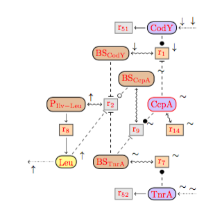
Graphically, reactions are drawn as boxed node. The fill-color of the box indicates whether the reaction is a candidate for knockout. The nodes of knockout candidates will be distinguished by a light orange color, while the others will be clored in gray.


    <!ATTLIST reaction %node;
    candidate    CDATA     #IMPLIED  >
  

candidate: if the attribute is present, the reaction is a candidate for knockout.

A species may interact in with the context via inflows and outflows.


    <!ELEMENT context  (input | output)> 
    <!ATTLIST   context %node; >
  

The three possible context elements are as follows:

context/input: an inflow from the context,

context/output: an outflow into the context,

The value of attribute spec of a context inflow or outflow is the identifier of the interacting species:


    <!ENTITY % species-identifier "
           spec      CDATA     #REQUIRED
           copy      CDATA     #IMPLIED      " >
    
    <!ELEMENT input   (#PCDATA)>
    <!ATTLIST input %species-identifier; >
    <!ELEMENT output  (#PCDATA)>
    <!ATTLIST output %species-identifier; >
   

Comments are given in latex format:


    <!ELEMENT comment      (#PCDATA)> 
    <!ATTLIST comment 
    latex	     CDATA    #IMPLIED 
    experiment   CDATA    #IMPLIED
    prediction   CDATA    #IMPLIED >
      

Arithmetic Expressions

References to real numbers (or real functions) are given by the following elements. There are constant, variables var, reference to control parameters param, references to the value of species conc either concentrations of amounts, references to the value of expression macros expr, and references to the speed of a reaction, i.e. to its kinetic-expression


<!ENTITY % reference "constant | param | conc | speed | var | expr ">

	   
<!ELEMENT constant  (#PCDATA)>
<!ATTLIST  constant 
	  id	      CDATA     #IMPLIED 
	  value    CDATA     #IMPLIED >

<!ELEMENT param  (#PCDATA)>
<!ATTLIST param
           id    CDATA     #REQUIRED >

<!ELEMENT expr  (#PCDATA) >
<!ATTLIST  expr
	   id          CDATA    #REQUIRED  >

<!ELEMENT var  (#PCDATA)>
<!ATTLIST  var 
           id	      CDATA     #IMPLIED >

<!ELEMENT conc  (#PCDATA)>
<!ATTLIST conc 
          spec    CDATA     #REQUIRED >

<!ELEMENT speed  (#PCDATA)>
<!ATTLIST speed
	  reaction    CDATA     #REQUIRED >

An arithmetic expression sometimes defines a real number in the simplest case. But in most cases, they define real-valued function. The atomic expressions are the references above. There are applications of buildin arithmetic functions mult, power, etc. The buildin functions are named as usual in MathML However, they are applied with a simplified syntax compared to MathML without using any apply elements.


<!ENTITY % expression "
          %reference; |
	  mult|sum|divide|minus|
	  sin|cos|tan|cot|
          sinh|cosh| tanh| coth|
          floor| ceiling|
  	  log| power|
	  time | inh | delay|
	  ifthenelse |
	  apply    ">

<!ELEMENT mult  (%expression;)*>
<!ELEMENT sum  (%expression;)*>
<!ELEMENT divide  ((%expression;),(%expression;))>
<!ELEMENT minus ((%expression;),(%expression;)?)>

<!ELEMENT power ((%expression;),(%expression;))>
<!ELEMENT log ((%expression;), (%expression;))>

<!ELEMENT sin (%expression;)>
<!ELEMENT cos (%expression;)>
<!ELEMENT tan (%expression;)>
<!ELEMENT cot (%expression;)>

<!ELEMENT sinh (%expression;)>
<!ELEMENT cosh (%expression;)>
<!ELEMENT tanh (%expression;)>
<!ELEMENT coth (%expression;)>

<!ELEMENT ceiling (%expression;)>
<!ELEMENT floor ((%expression;))>

Beside of the usual building operators from MathML, there are the following more specific operators:

  • time for the identity function
  • inh for the inhibition function with inh(x)=1/1+x
  • delay for delays in differential equations
  • ifthenelse for conditionals
  • apply for applying function defined in the network itself (rather than being buildin in MathML).

  <!ELEMENT time  (#PCDATA)>
  <!ELEMENT delay ((%expression;), (%expression;))> 
  <!ELEMENT inh (%expression;)>
  
  <!ELEMENT apply  ((%expression;)*)>
  <!ATTLIST  apply
           fun              CDATA     #REQUIRED
	   latex-look  CDATA     #IMPLIED >

Arithmetic expressions subsume conditionals ifthenelse that permit to define piecewise functions. They contain boolean expressions as conditions, which may compare real numbers for equality or ordering. Furthermore, Boolean expressions are closed under the boolean operators.


 <!ENTITY % boolexpression "eq | lt |  leq | and | or | not">

 <!ELEMENT ifthenelse
        ((%boolexpression;),(%expression;),(%expression;))>

Function Defintions

Functions can be defined by using lambda expressions possibly binding several variables at once.


<!ELEMENT function (lambda)>
<!ATTLIST  function %node;>

<!ELEMENT lambda ((bvar | %expression;)*)>
<!ELEMENT bvar  (#PCDATA)>
<!ATTLIST  bvar 
	  id	      CDATA     #IMPLIED >

A reaction may have a kinitic law that is described by the element kinetic-expression and defined by some artihmetic expression:

Kinetic Laws


<!ELEMENT kinetic-expression (%expression;)>
<!ATTLIST  kinetic-expression 
        angle      CDATA     #IMPLIED >
  

A way to describe kinetics in a partial manner is by using the element kinetics instead of kinetic-expression. This method is depricated. Named kinetics such as mass-action can be defined by arithmetic functions instead.

       
    <!ELEMENT kinetics    (#PCDATA) >
   
    <!ATTLIST kinetics
         id        CDATA     #IMPLIED
         expr      CDATA     #IMPLIED  
         mode      CDATA     #IMPLIED
         angle     CDATA     #IMPLIED  >
  

The kinetics is described either by the identifier @id or informally by the latex expression @expr. Whether the descriptor is exact or up to similarity is specifie by @mode.

@id: An identfier of a kinetics, which must have either of the following three values

  • exp : expression kinetics with constant equal to 1
  • ma : mass action kinetics with rate constant equal to 1
  • deac: deactivation kinetics with rate constant equal to 1

@expr: an arbitrary latex expression describing the kinetics. It may use the following predefined latex macros:

  • \BS{...} for binding sites,
  • \Prom{...} for promoters, and
  • \Op{...} for operons.

Other latex macros can be user defined by addition to the file Graph/Latex/macros.sty.

@mode: The interpretation mode may be either modulo similarity or exact. In the former case, the attribute mode must be absent, in the latter it must satisfy mode="equal".

@angle: The attribute angle says where the descriptor of the kinetics is annotated at the reaction node. If the id attribute is present, then the value of the annotation is the value of attribute expr.

Constraints:

  • exactely one of the attributes @id and @expr must be present.
  • the only possible value for @mode is equal.
  • the only possible values for @id are exp, ma, and deac

Modifiers and Reaction Complements

Reactions may have four kinds of modfiers: genral modifiers, inhibitors, activators, accelerators.


    <!ELEMENT modifier   (#PCDATA) >
    <!ATTLIST modifier    %species-reference; >
    <!ELEMENT inhibitor   (#PCDATA) >
    <!ATTLIST inhibitor   %species-reference; >
    <!ELEMENT activator   (#PCDATA) >
    <!ATTLIST activator   %species-reference; >
    <!ELEMENT accelerator (#PCDATA) >
    <!ATTLIST accelerator %species-reference; >
  

Beside of the modifiers there are three other kinds of reaction complements: reactants, products, and inhibited products (hiding a degradation reaction).


    <!ENTITY % reaction-complement "%species-reference;
        stoichiometry CDATA   #IMPLIED"  >
    <!ELEMENT reactant      (#PCDATA) >
    <!ATTLIST reactant      %reaction-complement; >
    <!ELEMENT product       (#PCDATA) >
    <!ATTLIST product       %reaction-complement; >
    <!ELEMENT product-inh   (#PCDATA) >
    <!ATTLIST product-inh   %reaction-complement; >
  

@stoichiometry: the value of the stoichiometry attribute it is computed automatically by the implementation. User defined stoichiometry values will be overwritten so that they become correct if necessary.

Macros for Expressions

We also have expressions defined by macros. These can be refered to by using the tag expr.

  
<!ELEMENT expression  (%expression;)>
<!ATTLIST  expression %node; >

Control Parameters and Events

A control parameter defines a trajectory by some arithmetic expression


<!ELEMENT parameter  (#PCDATA)>
<!ATTLIST  parameter %node; >

An event has a triger condition and a set of updates


  <!ELEMENT event (condition, (update)*)>
  <!ATTLIST  event 
        id	      CDATA     #IMPLIED  >

An trigger condition is a conjunction of equations and inequations


  <!ELEMENT condition (%boolexpression;)>
  
  <!ELEMENT eq  ((%expression;),(%expression;))>
  <!ELEMENT lt   ((%expression;),(%expression;))>
  <!ELEMENT leq ((%expression;),(%expression;))>
  <!ELEMENT and ((%boolexpression;)*)>
  <!ELEMENT or ((%boolexpression;)*)>
  <!ELEMENT not (%boolexpression;)>

we can update the concentrations of species and the values of parameters


  <!ELEMENT update ((conc|param), (%expression;))>
  <!ATTLIST  update>

Advanced Examples

The following examples illustrate some of the features discussed before, such as edgeclusters and splitpooints, but also some more advanced features.

Knockout predictions

We next come to an example of a bigger networks where edge clusters and copy node linked by splitpoins are needed to make the graph look nice. This is the graph of leucine network below.

There are reactions drawn in light orange for knockout candidate and others in medium orange for (unsafe) knockout predictions. While the knockout candididates are captured by the XML networks in the schema discussed before, the knockout prediction must be specified in an independent input file.

Leucine network

Branched chain amino acid network of B.~Subtilis.

Knockouts XML input file

    
<knockouts>
   <single>
      <knockout reaction="1" solution="2" />
      <knockout reaction="3" solution="3" />
      <knockout reaction="4" solution="4" />
      <knockout reaction="7" solution="5" />
      <knockout reaction="10" solution="6" />
      <knockout reaction="12" solution="7" />
      <knockout reaction="13" solution="8" />
      <knockout reaction="14" solution="9" />
      <knockout reaction="15" solution="10" />
      <knockout reaction="16" solution="11" />
      <knockout reaction="22" solution="12" />
      <knockout reaction="40" solution="13" />
      <knockout reaction="47" solution="14" />
   </single>
   <double/>
</knockouts>

Elementary Flux Analysis

In the graph of pyruvate metablic network below, we have annotated the result of an elementary flux analysis. The reactions are given a set of colors, that are annotated to the edges.

Pyruvate's metablic network.

Fluxes XML input file

    
<colors>
   <reaction id="47" thickness="2" >
      <color id="Apricot" />
      <color id="BlueGreen" />
      <color id="BlueViolet" />
      <color id="BrickRed" />
      <color id="BurntOrange" />
      <color id="Dandelion" />
      <color id="Fuchsia" />
      <color id="LimeGreen" />
   </reaction>
   <reaction id="48" thickness="2" >
      <color id="Apricot" />
   </reaction>
   <reaction id="14" thickness="2" >
      <color id="Aquamarine" />
      <color id="Cerulean" />
      <color id="DarkOrchid" />
      <color id="Green" />
      <color id="Magenta" />
   </reaction>
   <reaction id="15" thickness="2" >
      <color id="Aquamarine" />
   </reaction>
   <reaction id="12" thickness="2" >
      <color id="Bittersweet" />
      <color id="Cerulean" />
      <color id="DarkOrchid" />
      <color id="Green" />
      <color id="Magenta" />
   </reaction>
   <reaction id="13" thickness="2" >
      <color id="Bittersweet" />
   </reaction>
   <reaction id="16" thickness="2" >
      <color id="Black" />
      <color id="Cerulean" />
      <color id="DarkOrchid" />
      <color id="Green" />
      <color id="Magenta" />
   </reaction>
   <reaction id="17" thickness="2" >
      <color id="Black" />
   </reaction>
   <reaction id="8" thickness="2" >
      <color id="Blue" />
      <color id="Cerulean" />
      <color id="DarkOrchid" />
      <color id="Green" />
      <color id="Magenta" />
   </reaction>
   <reaction id="9" thickness="2" >
      <color id="Blue" />
   </reaction>
   <reaction id="159" thickness="2" >
      <color id="BlueGreen" />
      <color id="BlueViolet" />
      <color id="BrickRed" />
      <color id="BurntOrange" />
      <color id="Dandelion" />
      <color id="Fuchsia" />
      <color id="LimeGreen" />
   </reaction>
   <reaction id="5" thickness="2" >
      <color id="BlueGreen" />
      <color id="BrickRed" />
      <color id="Brown" />
      <color id="BurntOrange" />
      <color id="CadetBlue" />
      <color id="JungleGreen" />
   </reaction>
   <reaction id="7" thickness="2" >
      <color id="BlueGreen" />
      <color id="BrickRed" />
      <color id="Brown" />
      <color id="BurntOrange" />
      <color id="CadetBlue" />
      <color id="GreenYellow" />
   </reaction>
   <reaction id="10" thickness="2" >
      <color id="BlueGreen" />
      <color id="BlueViolet" />
      <color id="BrickRed" />
      <color id="Brown" />
      <color id="BurntOrange" />
      <color id="CadetBlue" />
      <color id="Cyan" />
      <color id="Dandelion" />
      <color id="ForestGreen" />
      <color id="Fuchsia" />
      <color id="Gray" />
      <color id="LimeGreen" />
   </reaction>
   <reaction id="50" thickness="2" >
      <color id="BlueGreen" />
      <color id="BrickRed" />
      <color id="Brown" />
      <color id="CarnationPink" />
      <color id="Dandelion" />
      <color id="DarkOrchid" />
      <color id="Fuchsia" />
      <color id="Green" />
   </reaction>
   <reaction id="51" thickness="2" >
      <color id="BlueGreen" />
      <color id="BrickRed" />
      <color id="Brown" />
      <color id="CadetBlue" />
      <color id="CarnationPink" />
      <color id="Cyan" />
      <color id="Dandelion" />
      <color id="DarkOrchid" />
      <color id="ForestGreen" />
      <color id="Fuchsia" />
      <color id="Green" />
   </reaction>
   <reaction id="53" thickness="2" >
      <color id="BlueGreen" />
      <color id="BlueViolet" />
      <color id="BurntOrange" />
      <color id="CadetBlue" />
      <color id="Cerulean" />
      <color id="CornflowerBlue" />
   </reaction>
   <reaction id="56" thickness="2" >
      <color id="BlueGreen" />
      <color id="BlueViolet" />
      <color id="BrickRed" />
      <color id="Brown" />
      <color id="BurntOrange" />
      <color id="CadetBlue" />
      <color id="Cerulean" />
      <color id="ForestGreen" />
      <color id="Fuchsia" />
      <color id="Goldenrod" />
      <color id="Green" />
   </reaction>
   <reaction id="149" thickness="2" >
      <color id="BlueViolet" />
      <color id="Cyan" />
      <color id="Dandelion" />
      <color id="DarkOrchid" />
      <color id="Emerald" />
      <color id="ForestGreen" />
      <color id="Fuchsia" />
      <color id="LimeGreen" />
      <color id="Magenta" />
   </reaction>
   <reaction id="2" thickness="2" >
      <color id="BlueViolet" />
      <color id="BurntOrange" />
      <color id="Cerulean" />
      <color id="Lavender" />
      <color id="LimeGreen" />
      <color id="Magenta" />
   </reaction>
   <reaction id="3" thickness="2" >
      <color id="BrickRed" />
      <color id="Brown" />
      <color id="CarnationPink" />
      <color id="Lavender" />
   </reaction>
   <reaction id="146" thickness="2" >
      <color id="Brown" />
      <color id="CadetBlue" />
      <color id="Cerulean" />
      <color id="Cyan" />
      <color id="DarkOrchid" />
      <color id="ForestGreen" />
      <color id="Green" />
      <color id="Magenta" />
   </reaction>
   <reaction id="46" thickness="2" >
      <color id="Brown" />
      <color id="CadetBlue" />
      <color id="Cyan" />
      <color id="ForestGreen" />
   </reaction>
   <reaction id="49" thickness="2" >
      <color id="Brown" />
      <color id="CadetBlue" />
      <color id="Cyan" />
      <color id="ForestGreen" />
   </reaction>
   <reaction id="54" thickness="2" >
      <color id="CarnationPink" />
      <color id="CornflowerBlue" />
      <color id="Cyan" />
      <color id="Dandelion" />
      <color id="DarkOrchid" />
      <color id="Emerald" />
   </reaction>
   <reaction id="500" thickness="2" >
      <color id="Cerulean" />
      <color id="DarkOrchid" />
      <color id="Green" />
      <color id="Magenta" />
   </reaction>
   <reaction id="1" thickness="2" >
      <color id="Cerulean" />
      <color id="DarkOrchid" />
      <color id="Green" />
      <color id="Magenta" />
   </reaction>
   <reaction id="18" thickness="2" >
      <color id="Cerulean" />
      <color id="DarkOrchid" />
      <color id="Green" />
      <color id="Magenta" />
   </reaction>
   <reaction id="4" thickness="2" >
      <color id="Cyan" />
      <color id="Dandelion" />
      <color id="DarkOrchid" />
      <color id="Emerald" />
      <color id="JungleGreen" />
      <color id="LimeGreen" />
      <color id="Magenta" />
   </reaction>
   <reaction id="6" thickness="2" >
      <color id="Cyan" />
      <color id="Dandelion" />
      <color id="DarkOrchid" />
      <color id="Emerald" />
      <color id="GreenYellow" />
      <color id="LimeGreen" />
      <color id="Magenta" />
   </reaction>
   <reaction id="55" thickness="2" >
      <color id="Emerald" />
      <color id="Goldenrod" />
   </reaction>
   <reaction id="11" thickness="2" >
      <color id="Gray" />
   </reaction>
</colors>

Solution Annotations for Abstract Interpretation

We next show that reaction nodes of network's graph can be annotated with a solution of a difference constraint, that was derived from the network's steady state equation by abstract interpretation.

A solution annotated to the network's graph.

Solutions XML input file

    
<results>
   <variables>
      <var kind="global" >o_1</var>
      <var kind="global" >o_7</var>
      <var kind="global" >o_8</var>
      <var kind="global" >o_14</var>
      <var kind="global" >v_1</var>
      <var kind="global" >v_7</var>
      <var kind="global" >v_9</var>
      <var kind="global" >v_14</var>
      <var kind="global" >x_CodY</var>
      <var kind="global" >x_TnrA</var>
      <var kind="global" >y_Leu</var>
      <var kind="global" >z_BSCcpA</var>
      <var kind="global" >z_BSCodY</var>
      <var kind="global" >z_BSTnrA</var>
      <var kind="global" >z_CcpA</var>
      <var kind="global" >z_CodY</var>
      <var kind="global" >z_Leu</var>
      <var kind="global" >z_PIlv_Leu</var>
      <var kind="global" >z_TnrA</var>
  </variables>
   <result>
      <variables>
         <var kind="global" >v_1</var>
         <var kind="global" >x_CodY</var>
         <var kind="global" >y_Leu</var>
         <var kind="global" >z_BSCodY</var>
         <var kind="global" >z_CodY</var>
         <var kind="global" >z_Leu</var>
         <var kind="global" >z_PIlv_Leu</var>
      </variables>
      <solution v_1="Do" x_CodY="Do" y_Leu="Up" z_BSCodY="Do" z_CodY="Do" z_Leu="Up" z_PIlv_Leu="Up" >
         <weight>70</weight>
         <position>2</position>
      </solution>
   </result>
</results>

A network with complete kinetic information

Without any extra files, we can annotate all reaction of a network with kinetic expressions, similarly to what is done in SBML.

A part of the Smad network.

Smad XML network

    
<network id="bio" scale=".8" >

  <!-- species -->

  <actor id="A" x="0.3" y="1" latex-look="G4_c" comment="cytoplasmic EGFP-Smad2/Smad4 complex" />
  <actor id="C" x="2.7" y="1" latex-look="pG_c" comment="cytoplasmic phosphorilated EGFP-Smad2 complex" />
  <actor id="X" x="4.5" y="1" latex-look="S4_c" comment="cytoplasmic Smad4" />
  <actor id="E" x="6.3" y="1" latex-look="pS2_c" comment="cytoplasmic phosphorilated Smad2" />
  <actor id="W" x="8.7" y="1" latex-look="S24_c" comment="cytoplasmic Smad2/Smad4 complex" />

  <actor id="B" x="0.3" y="-3" latex-look="G4_n" comment="nuclear EGFP-Smad2/Smad4 complex" />
  <actor id="D" x="2.7" y="-3" latex-look="pG_n" comment="nuclear phosphorilated EGFP-Smad2 complex" />
  <actor id="Y" x="4.5" y="-3" latex-look="S4_n" comment="nuclear Smad4" />
  <actor id="F" x="6.3" y="-3" latex-look="pS2_n" comment="nuclear phosphorilated Smad2" />
  <actor id="Z" x="8.7" y="-3" latex-look="S24_n" comment="nuclear Smad2/Smad4 complex" />

  <!-- reactions  -->


    <reaction id="22" x="1.5" y="2" comment="Formation of \M{A}" >
    <kinetics expr="C \kon\z C\z X" angle="90" />
    <product spec="A" />
    <reactant spec="C" />
    <reactant spec="X" />
  </reaction>

  <reaction id="-22" x="1.5" y="0" comment="Decomposition of \M{A}" >
    <kinetics expr="C \koff\z A" angle="-90" />
    <reactant spec="A" />
    <product spec="C" />
    <product spec="X" />
  </reaction>

  <reaction id="5" x="7.5" y="2" comment="Formation of complex \M{W}" >
    <kinetics expr="C \kon\z X\z E" angle="90" />
    <reactant spec="X" />
    <reactant spec="E" />
    <product spec="W" /> 
  </reaction>

  <reaction id="-5" x="7.5" y="0" comment="Decomposition of complex \M{W}" >
    <kinetics expr="C \koff\z W" angle="-90" />
    <product spec="X" />
    <product spec="E" />
    <reactant spec="W" /> 
  </reaction>
  

    <reaction id="23" x="1.5" y="-2" comment="Formation of \M{B}" >
    <kinetics expr="N \kon\z D\z Y" angle="90" />
    <product spec="B" />
    <reactant spec="D" />
    <reactant spec="Y" />
  </reaction>

  <reaction id="-23" x="1.5" y="-4" comment="Decomposition of \M{B}" >
    <kinetics expr="N \koff\z B" angle="-90" />
    <reactant spec="B" />
    <product spec="D" />
    <product spec="Y" />
  </reaction>

  <reaction id="6" x="7.5" y="-2" comment="Formation of complex \M{Z}" >
    <kinetics expr="\k{on} N\z Y \z F" angle="90" />
    <reactant spec="Y" />
    <reactant spec="F" />
    <product spec="Z" /> 
  </reaction>

  <reaction id="-6" x="7.5" y="-4" comment="Decomposition of complex \M{Z}" >
    <kinetics expr="\k{off} N \z Z" angle="-90" />
    <product spec="Y" />
    <product spec="F" />
    <reactant spec="Z" /> 
  </reaction>
  

    <reaction id="1" x="4" y="-1" comment="Shuttling of \M{X} into nucleus" >
    <kinetics expr="\k{in}\z X" angle="180" />
    <product spec="Y" />
    <reactant spec="X" /> 
  </reaction>
  
  <reaction id="-1" x="5" y="-1" comment="Shuttling of \M{Y} into cytoplasm" >
    <kinetics expr="\k{out}\z{Y}" angle="0" />
    <product spec="X" />
    <reactant spec="Y" /> 
  </reaction>
  
  <reaction id="7" x="8.7" y="-1" comment="Shuttling of \M{W} into nucleus" >
    <kinetics expr="\k{in}C I F \z W" angle="0" />
    <product spec="Z" />
    <reactant spec="W" /> 
  </reaction>
 
  
</network>