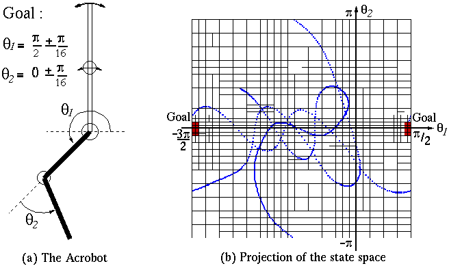

The state space :
The Acrobot is defined by the 4-dimensional state x=(theta1, theta2, theta1_dot, theta2_dot)The control space :
where (theta1, theta2) are the angles (see figure) and (theta1_dot, theta2_dot) are their velocities.
The control u is a 1-dimensional variable that takes aThe state dynamics :
finite number of possible values between -max_torque and +max_torque.
It represents the torque applied to the elbow.
The state dynamics is defined by the differential equation :The reinforcement functions :
dx
-- = f(x,u)
dt
in the deterministic case, and by the stochastic diff. eq. :dx = f(x,u) dt + s(x,u) dw
in the stochastic case. Here dw is a Wiener process.
(The formulation of the stochasticity is explained is the
function acrobot_noise).
The current and terminal reinforcement functions are describedCode in C :
in the functions :
- acrobot_current_reinf
- acrobot_terminal_reinf
/* Definition of some constants and basic functions
*/
#define max_torque 2.0
#define friction 0.0
#define m1 1.0 /* Mass of shoulder-to-elbow joint */
#define m2 1.0 /* Mass of elbow-to-hand joint */
#define l 1.0 /* Distance from shoulder to elbow AND Distance from
elbow to hand */
#define GRAVITY 9.81
/* This is the state dynamics.
Inputs :
p1 = state[0];
p2 = state[1];
v1 = state[2];
v2 = state[3];
t1 = action;
t2 = 0;
a1 = 0;
a2 = 0;
joint_accns(p1, v1, p2, v2, t1, t1, &a1, &a2);
f[0]=v1;
f[1]=v2;
f[2]=a1;
f[3]=a2;
}
/* This is the stochastic part.
The stochastic differential equation :
dx = f(x,u) dt + s(x,u) dw
includes 2 part :
eig_vect[0][0]=1;
eig_vect[1][0]=0;
eig_vect[2][0]=0;
eig_vect[3][0]=0;
eig_vect[0][1]=0;
eig_vect[1][1]=1;
eig_vect[2][1]=0;
eig_vect[3][1]=0;
eig_vect[0][2]=0;
eig_vect[1][2]=0;
eig_vect[2][2]=1;
eig_vect[3][2]=0;
eig_vect[0][3]=0;
eig_vect[1][3]=0;
eig_vect[2][3]=0;
eig_vect[3][3]=1;
}
/* The current reinforcement (here 0 everywhere)
*/
double acrobot_current_reinf(task *tsk,
double *state, double action, double seconds)
{
return 0;
}
/* The terminal reinforcement : this function
is called only when the systems reached the goal
*/
double acrobot_terminal_reinf(task *tsk,
double *state)
{
return 1.0;
}
/* Now here are some internal functions
*/
/*
pi = angle of ith joint
vi = angular velocity of ith joint
ti = torque applied to ith joint
ai = angular acceleration of ith joint
Fu et al's robot book gives that
t = D a + h + k
where t , a are vectors, of torques and accns
respectively.
D IS A SYMMETRIC 2X2 MATRIX
h and k are vectors
*/
void joint_accns (double p1, double v1,
double p2, double v2, double t1, double t2, double *res_a1, double *res_a2)
{
double c1 = cos(p1);
double c2 = cos(p2);
double c12 = cos(p1 + p2);
double s2 = sin(p2);
double lsqd = l * l;
double m2_lsqd = m2 * lsqd;
double m2gl = m2 * GRAVITY * l;
double d11 = 1.0/3 * m1 * lsqd + (4.0/3 + c2) * m2_lsqd;
double d12 = (1.0/3 + 1.0/2 * c2) * m2_lsqd;
double d22 = 1.0/3 * m2_lsqd;
double h1 = -m2_lsqd * s2 * v2 * ( 1.0/2 * v2 + v1);
double h2 = 1.0/2 * s2 * v1 * v1 * m2_lsqd;
double k2 = 1.0/2 * m2gl * c12;
double k1 = 1.0/2 * m1 * GRAVITY * l * c1 + k2 + m2gl * c1;
double y1 = t1 - h1 - k1;
double y2 = t2 - h2 - k2;
double b = d12 * d12 - d11 * d22;
if ( fabs(b) < 1e-20 ) my_error("tarm.c singularity");
*res_a2 = (d12 * y1 - d11 * y2) / b;
*res_a1 = (d12 * y2 - d22 * y1) / b;
}
/* Gives the x and y coordinates of the elbow
in (*j1_x,*j1_y)
and the hand in (*j2_x,*j2_y). So a simple stick
figure drawing of
the arm is just two lines, the first from (0,0)
to (j1x,j1y). The
second from (j1x,j1y) to (j2x,j2y) */
void arm_kinematics (double p1, double
p2, double *j1_x, double *j1_y, double *j2_x, double *j2_y)
{
double c1 = cos(p1);
double c12 = cos(p1 + p2);
double s1 = sin(p1);
double s12 = sin(p1 + p2);
*j1_x = l * c1;
*j1_y = l * s1;
*j2_x = *j1_x + l * c12;
*j2_y = *j1_y + l * s12;
}
Some numerical values :