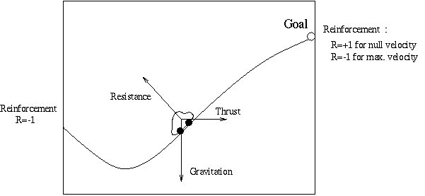

The state space :
The car is defined by the 2-dimensional state x=(y,v)The control space :
where y is its position and v its velocity.
The control u is a 1-dimensional variable that takes aThe state dynamics :
finite number of possible values between u_min and u_max.
It represents the thrust applied to the car.
The state dynamics is defined by the differential equation :The reinforcement functions :
dx
-- = f(x,u)
dt
in the deterministic case, and by the stochastic diff. eq. :dx = f(x,u) dt + s(x,u) dw
in the stochastic case. Here dw is a Wiener process.
(The formulation of the stochasticity is explained is the
function hillcar_noise).
The current and terminal reinforcement functions are describedCode in C :
in the functions :
- hillcar_current_reinf
- hillcar_terminal_reinf
/* Definition of some constants and basic functions
*/
#define A 1.0
#define B 5.0
#define C 0.0
#define MASS 1.0
#define GRAVITY 9.81
#define f1(x) ((x) * ((x) + 1.0))
#define f1_dashed2(x) (2.0 * (x) + 1.0)
#define f2(x) (A * (x) / sqrt(1.0 + B * (x) * (x)))
#define f(x) (((x) < C) ? f1(x):f2(x))
#define f_dashed(x) (((x) < C) ? f1_dashed2(x) : f2_dashed2(x))
double f2_dashed2(double x)
{
double alpha = sqrt(1.0 + B * x * x);
return( A / (alpha * alpha * alpha) );
}
/* This is the state dynamics.
Inputs :
x = state[0];
q = f_dashed(x);
p = 1.0 + (q * q);
acc = (action / (MASS * sqrt(p))) - (GRAVITY * q / p);
f[0] = state[1];
f[1] = acc;
}
/* This is the stochastic part.
The stochastic differential equation :
dx = f(x,u) dt + s(x,u) dw
includes 2 part :
eig_vect[0][0]=1;
eig_vect[1][0]=0;
eig_vect[0][1]=0;
eig_vect[1][1]=1;
}
/* The current reinforcement (here 0 everywhere)
*/
double hillcar_current_reinf(task *tsk,
double *state, double action, double seconds)
{
return 0;
}
/* The terminal reinforcement : this function is called only when the systems exits from the state space.
Some numerical values :